构建一个分类器需要经过如下几个步骤:
- 加载并可视化数据
- 图像预处理
- 特性提取
- 图像分类并查看错误的情况
1. 加载并可视化数据
为了对图像集进行解析和处理,第一步当然是要了解我们的目标,首先获取一个感性的认识,然后分析其特点
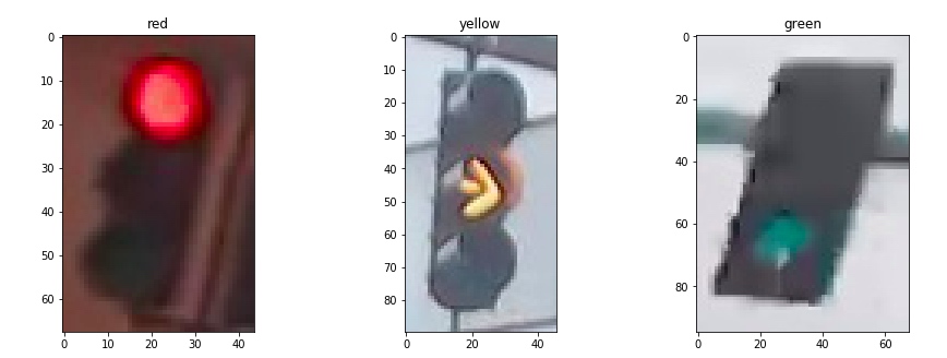
我们首先从图像集里面过滤出三种颜色的信号灯,然后各取一张进行显示:
red_images = [img for img in IMAGE_LIST if img[1]=='red']
yellow_images = [img for img in IMAGE_LIST if img[1]=='yellow']
green_images = [img for img in IMAGE_LIST if img[1]=='green']


f,(ax1,ax2,ax3) = plt.subplots(1,3,figsize=(15,5))
ax1.imshow(red_images[0][0])
ax2.imshow(yellow_images[0][0])
ax3.imshow(green_images[0][0])
ax1.set_title(red_images[0][1])
ax2.set_title(yellow_images[0][1])
ax3.set_title(green_images[0][1])
2. 图像预处理
通过观察,可以发现几点关键信息:[^1]
- 图片尺寸不一致
- 图片光照条件不一致
为此我们需要对图像进行预处理:
- 标准化
- one-hot 编码
#标准化
def standardize_input(image):
    standard_im = np.copy(image)
    standard_im = cv.Resize(standard_im,(32,32))
    return standard_im
#one-hot 编码
def one_hot_encode(label):
    if(label=='red'):
        one_hot_encoded = [1,0,0]
    elif(label=='yellow'):
        one_hot_encoded = [0,1,0]
    elif(label=='green'):
        one_hot_encoded = [0,0,1]
    return one_hot_encoded
随后将图像集传入将所有图像进行标准化
def standardize(image_list):
    standard_list = []
    for item in image_list:
        image = item[0]
        label = item[1]

        #标准化一幅图像
        standardized_im = standardize_input(image)

        # 编码
        one_hot_label = one_hot_encode(label)

      standard_list.append((standardized_im, one_hot_label))

    return standard_list


STANDARDIZED_LIST = standardize(IMAGE_LIST)
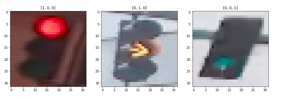
将STANDARDIZED_LIST中的结果选择其一打印出来
3. 特性提取
抽取特征
- 亮度特征
- 颜色特征
- ....
1. 亮度特征
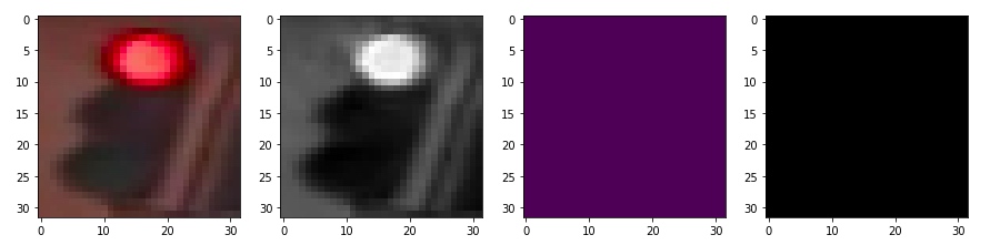
首先我们将图像转换为 hsv 颜色空间
image_num = 0
test_im = STANDARDIZED_LIST[image_num][0]
test_label = STANDARDIZED_LIST[image_num][1]

# Convert to HSV
hsv = cv2.cvtColor(test_im, cv2.COLOR_RGB2HSV)

# Print image label
print('Label [red, yellow, green]: ' + str(test_label))

# HSV channels
h = hsv[:,:,0]
s = hsv[:,:,1]
v = hsv[:,:,2]

f, (ax1, ax2, ax3, ax4) = plt.subplots(1, 4, figsize=(20,10))
ax1.set_title('Standardized image')
ax1.imshow(test_im)
ax2.set_title('H channel')
ax2.imshow(h, cmap='gray')
ax3.set_title('S channel')
ax3.imshow(s, cmap='gray')
ax4.set_title('V channel')
ax4.imshow(v, cmap='gray')
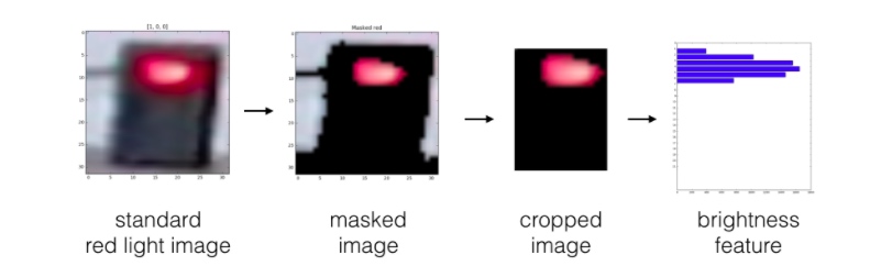
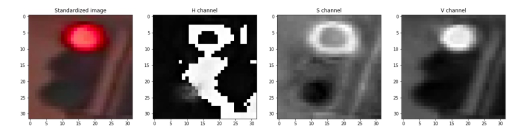 由此可以看到,value 最能作为图像的特征,但是首先我们需要对图像进行预处理,这里的预处理指的是,我们需要对图像进行一些裁剪,保证信号灯部分占据主体。随后,将图像分割为上中下三部分,分别求对应部分像素value值的和,确定最亮的部分位于图像上中下哪个部分,以此作为信号灯判断的依据。
def show_img_bright(rgb,hsv,mask,masked):
    fig,(ax1,ax2,ax3,ax4) = plt.subplots(1,4,figsize=(10,10))
    ax1.imshow(rgb)
    ax2.imshow(hsv[:,:,2],cmap='gray')
    ax3.imshow(mask,cmap='gray')
    ax4.imshow(masked[:,:,2],cmap='gray')


def apply_bright_mask(mask,rgb_image):
    masked_hsv_image = np.copy(rgb_image)
    masked_hsv_image[mask == 0] = [0, 0, 0]
    return masked_hsv_image

def apply_resize(rgb_image):
    v = 5
    h = 10
    return rgb_image[v:-v,h:-h,:]

def calculate_brightness(hsv_img):

    height  = hsv_img.shape[0]
    width = hsv_img.shape[1]

    block_height = height//3

    top_sum = np.sum(hsv_img[:block_height,:,2])
    mid_sum = np.sum(hsv_img[block_height:block_height*2,:,2])
    bot_sum = np.sum(hsv_img[block_height*2:block_height*3,:,2])
    return [top_sum,mid_sum,bot_sum]


def create_feature_brightness(rgb_image):
    hsv_img = cv2.cvtColor(rgb_image, cv2.COLOR_RGB2HSV)
    lower_hsv = np.array(210)
    upper_hsv = np.array(255)
    mask=cv2.inRange(hsv_img[:,:,2],lower_hsv,upper_hsv)
    masked_hsv_image = apply_bright_mask(mask,rgb_image)
    resized_masked_img = apply_resize(masked_hsv_image)
    #show_img_bright(rgb_image,hsv_img,mask,resized_masked_img)
    feature = calculate_brightness(resized_masked_img)

    #print(feature)
    return feature
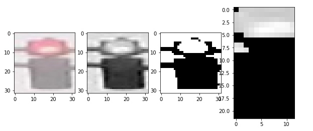
至此,我们得到了图像的亮度特征。
但是作为交通灯,显然有亮度是不行的,因此我们再加入一个颜色特征
2. 颜色特征
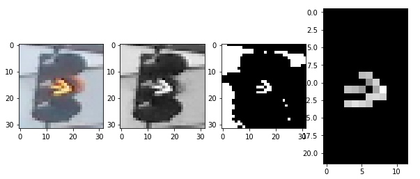
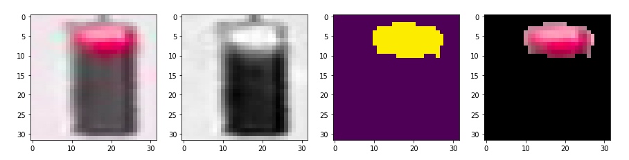
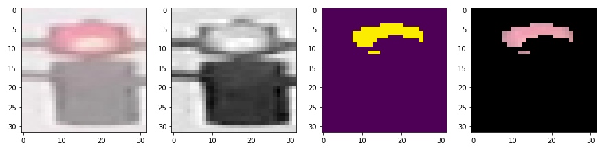
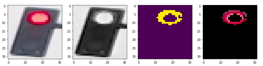
既然是信号灯,颜色自然是一个明显的特征,这里的思路是,首先转换为 hsv颜色空间,然后基于不同颜色对图像做 mask,将三种颜色对应的部分扣出来,分别计算其像素的和,最大的就是对应颜色
def show_img(rgb,hsv,mask,masked):
fig,(ax1,ax2,ax3,ax4) = plt.subplots(1,4,figsize=(20,20))
ax1.imshow(rgb)
ax2.imshow(hsv[:,:,2],cmap='gray')
ax3.imshow(mask)
ax4.imshow(masked)
def apply_mask(mask,rgb_image):
masked_hsv_image = np.copy(rgb_image)
masked_hsv_image[mask == 0] = [0, 0, 0]
return masked_hsv_image
def get_sum_red(rgb_image):
hsv = cv2.cvtColor(rgb_image, cv2.COLOR_RGB2HSV)
lower_hsv = np.array([120, 50, 120])
upper_hsv = np.array([180, 255, 255])
mask=cv2.inRange(hsv,lower_hsv,upper_hsv)
masked_hsv_image=apply_mask(mask,rgb_image)
total = np.sum(masked_hsv_image[:,:,:])
#show_img(rgb_image,hsv,mask,masked_hsv_image)
return total
def get_sum_yellow(rgb_image):
hsv = cv2.cvtColor(rgb_image, cv2.COLOR_RGB2HSV)
lower_hsv = np.array([10, 50, 120])
upper_hsv = np.array([70, 255, 255])
mask=cv2.inRange(hsv,lower_hsv,upper_hsv)
masked_hsv_image=apply_mask(mask,rgb_image)
total = np.sum(masked_hsv_image[:,:,:])
#show_img(rgb_image,hsv,mask,masked_hsv_image)
return total
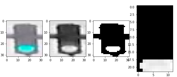
def get_sum_green(rgb_image):
hsv = cv2.cvtColor(rgb_image, cv2.COLOR_RGB2HSV)
lower_hsv = np.array([70, 50, 120])
upper_hsv = np.array([100, 255, 255])
mask=cv2.inRange(hsv,lower_hsv,upper_hsv)
masked_hsv_image=apply_mask(mask,rgb_image)
total = np.sum(masked_hsv_image[:,:,:])
#show_img(rgb_image,hsv,mask,masked_hsv_image)
return total
# (Optional) Add more image analysis and create more features
def create_feature_color(rgb_image):
red_total = get_sum_red(rgb_image)
yellow_total = get_sum_yellow(rgb_image)
green_total = get_sum_green(rgb_image)
feature=[0,0,0]
return [red_total,yellow_total,green_total]
查看一下利用hsv 三个分量阈值过滤的效果
如果是用黄色过滤
 用绿色过滤
用绿色过滤
4. 图像分类并查看错误的情况
1. 应用特征进行估计
这里要注意的是如何运用多个特征进行估计。
Fully-connected layer A fully-connected layer's job is to connect the input it sees to a desired form of output. As an example, say we are sorting images into two classes: day and night, you could give a fully-connected layer a set of feature maps and tell it to use a combination of these features (multiplying them, adding them, combining them, etc.) to output a prediction: whether a given image is likely taken during the "day" or "night." This output prediction is sometimes called the output layer.
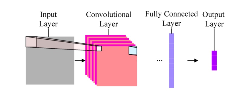
我们可以认为我们已经使用了两种不同的方法(convolutional layer)得到了两个特征,现在需要再 fully connected layer 将不同的特征进行组合。
注意:特征指的是特征提取的原始结果,并非基于其得出的 one-hot 编码。
在这个项目里,我采取的是将两种特征(颜色和亮度)进行求和,然后使用合成后的特征进行预测,得到 one-hot 编码
def predict(feature):
    predicted_label = [0,0,0]
    if feature[0] > feature[1] and feature[0] > feature[2]:
        predicted_label = [1,0,0]
    elif feature[1] > feature[0] and feature[1] > feature[2]:
        predicted_label = [0,1,0]
    elif feature[2] > feature[0] and feature[2] > feature[1]:
        predicted_label = [0,0,1]
    return predicted_label


def estimate_label(rgb_image):
    predicted_label = [0,0,0]

    #颜色特征
    color_feature = create_feature_color(rgb_image)
    #亮度特征
    bright_feature = create_feature_brightness(rgb_image)
    #print(color_feature," ",bright_feature)

    #求和特征
    feature = [i+j for i,j in zip(color_feature,bright_feature)]

    predicted_label = predict(feature)

    return predicted_label
2. 图像分类并计算失误率
使用模型进行分类并收集错误的结果用于评估
def get_misclassified_images(test_images):
    "对图像集进行分类并获取被错误分类的图像"
    misclassified_images_labels = []

    for image in test_images:
        im = image[0]
        true_label = image[1]

        predicted_label = estimate_label(im)

        if(predicted_label != true_label):
            misclassified_images_labels.append((im, predicted_label, true_label))

    return misclassified_images_labels
#原始图像集
TEST_IMAGE_LIST = helpers.load_dataset(IMAGE_DIR_TEST)
#标准化尺寸图像集
STANDARDIZED_TEST_LIST = standardize(TEST_IMAGE_LIST)
#错误分类的图像集
MISCLASSIFIED = get_misclassified_images(STANDARDIZED_TEST_LIST)


total = len(STANDARDIZED_TEST_LIST)
num_correct = total - len(MISCLASSIFIED)
accuracy = num_correct/total

print('Accuracy: ' + str(accuracy))
print("Number of misclassified images = " + str(len(MISCLASSIFIED)) +' out of '+ str(total))
结果如下:
Accuracy: 0.9831649831649831 Number of misclassified images = 5 out of 297
使用两个特征的分类结果,可能优于一个特征,但也可能因为不当的组合产生劣化的效果。[^2]
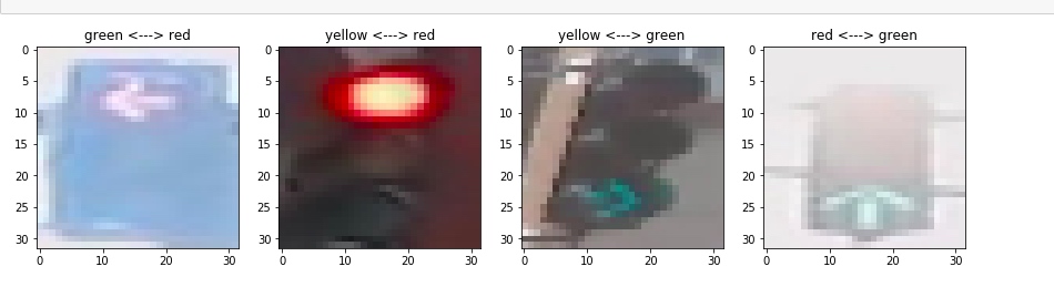
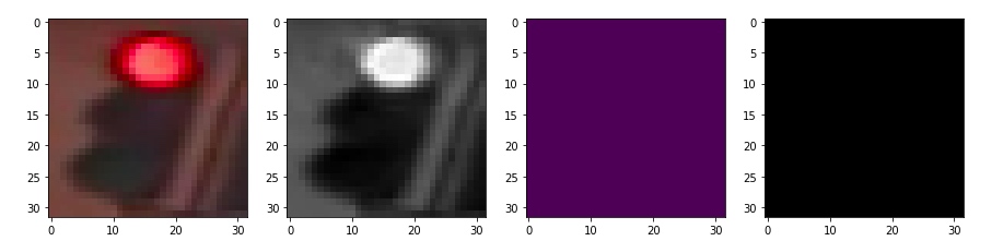
3. 查看错误分类的图像
def get_label_string(label):
    if label[0]==1:
        return "red"
    elif label[1]==1:
        return "yellow"
    elif label[2]==1:
        return "green"
    else:
        return "miss"


img_num = len(MISCLASSIFIED)
cols = 4
rows = img_num%cols
fig, axes = plt.subplots(nrows=rows, ncols=cols,figsize=(15,10))

#绘制子图, subplots 返回的axes 是一个 nrows*ncols 的矩阵

fig, axes = plt.subplots(nrows=img_num, ncols=1,figsize=(20,50))

#给每一个子轴赋值
#如果 axes 不是向量而是矩阵,则必须迭代axes.flat)
for data,axe in zip(MISCLASSIFIED,axes.flat):
    img=data[0]
    label=data[1]
    true_label = data[2]
    axe.imshow(img)
    predict_label = get_label_string(label)
    true_label = get_label_string(true_label)

    axe.set_title(predict_label+" <---> "+true_label)

plt.show()
被错误分类的4幅图像如下[^3]