卷积神经网络
- 如果我们已经知晓数据集的某些特征,学习可以变得更容易,例如,如果我们知道,颜色不是决定字母的因素,我们则可以采取灰度图像而非RGB图像
- 如果我们想判断图片中是否有猫,不指定猫的位置会让学习更简单
- 如果我们的神经网络试图理解一个句子,句子中反复出现的单词kitten,基本上和它出现的位置无关
1. 统计不变量与贡献权重
在上面两个例子中,目标中有部分信息可以反复利用,而不需要重新学习。我们可以通过共享权重来利用这一点。
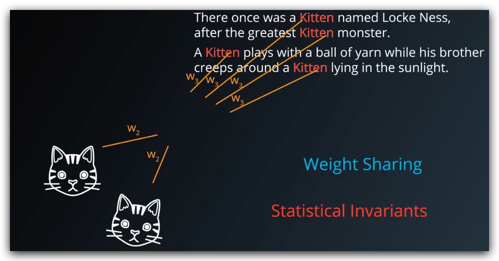
当我们知道,两个输入中可能包含相同的信息时,我们可以共享它们的权重,并且利用这些输入,共同训练权重。 统计不变量指的是基本上不会随时空变换的统计量。
2. 卷积神经网络
1. 术语
- 过滤器
- 步长
- patch
- Padding
2. 过滤器(kernel)
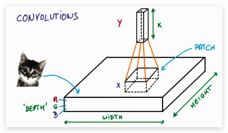
过滤器的深度是指过滤器的个数,每个过滤器提取特定的特征,那么特征的数量就是深度,假设深度为k,则该patch在下一层连接k个感知元。
为什么要连接多个感知元呢?因为一个patch可能有多个我们感兴趣的特征。
3. Feature Map Sizes
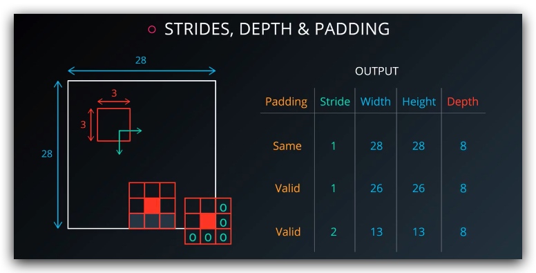
4. Padding
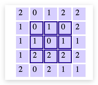
5*5的grid中,创建一个3*3的kernel,步长为1 的情况下,则下一层的维度是3*3(在任意方向只能通过移动,创建3个patch)
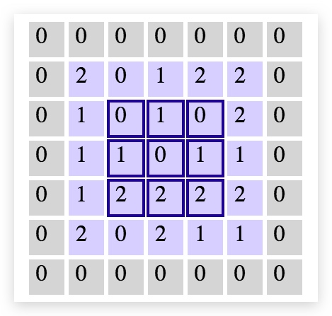
为了不减少维度,我们可以对grid进行补0操作,使的我们能够创建足够多的patch来保持维度不变
5. 卷积层尺寸
我们必须能够知道,每层网络的大小,以便知晓模型的规模,在尺寸和性能上做出取舍
- 输入层 width 为 W , height 为 H
- 卷积层的过滤器大小为 F
- 步长为 S
- padding 为 P
- 深度,即过滤器的个数为 K
则,下一层的尺寸为:
W_out =[ (W−F+2P)/S] + 1H_out = [(H-F+2P)/S] + 1D_out = K- 下一层的尺寸为
W_out * H_out * D_out
练习
Setup H = height, W = width, D = depth
- We have an input of shape 32x32x3 (HxWxD)
- 20 filters of shape 8x8x3 (HxWxD)
- A stride of 2 for both the height and width (S)
- With padding of size 1 (P)
D_out = K = 20
W_out =[ (32−8+2)/2] + 1 = 14
H_out =[ (32−8+2)/2] + 1 = 14
但是下面一段代码,conv的输出维度是[1, 16, 16, 20],而不是[1, 14, 14, 20],这和tf添加padding的机制有关,可以看这里
input = tf.placeholder(tf.float32, (None, 32, 32, 3))
filter_weights = tf.Variable(tf.truncated_normal((8, 8, 3, 20))) # (height, width, input_depth, output_depth)
filter_bias = tf.Variable(tf.zeros(20))
strides = [1, 2, 2, 1] # (batch, height, width, depth)
padding = 'SAME'
conv = tf.nn.conv2d(input, filter_weights, strides, padding) + filter_bias
简单来讲: SAME Padding: out_height = ceil(float(in_height) / float(strides[1])) out_width = ceil(float(in_width) / float(strides[2])) VALID Padding out_height = ceil(float(in_height - filter_height + 1) / float(strides[1])) out_width = ceil(float(in_width - filter_width + 1) / float(strides[2]))
参数个数计算
按照上述的输入输出结果(Output Layer 14x14x20 (HxWxD)),计算参数的个数:
- 如果不共享参数,则每一层参数个数为
(8 * 8 * 3 + 1) * (14 * 14 * 20) = 756560(+1是bias) - 如果是共享参数的CNN,则参数个数为
(8 * 8 * 3 + 1) * 20 = 3840 + 20 = 3860
我们可以看出,共享参数则不需要在输出层的每个W*H上再去学习,只需要乘上深度即可。
6. 卷积神经网络的可视化
第一层
So, the first layer of our CNN clearly picks out very simple shapes and patterns like lines and blobs.
第二层
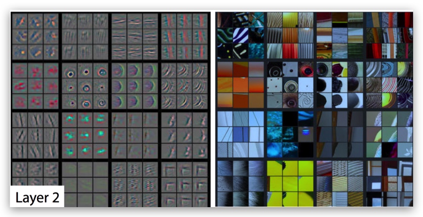
As you see in the image above, the second layer of the CNN recognizes circles (second row, second column), stripes (first row, second column), and rectangles (bottom right).
第三层
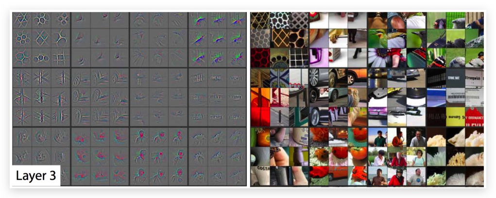
The third layer picks out complex combinations of features from the second layer. These include things like grids, and honeycombs (top left), wheels (second row, second column), and even faces (third row, third column).
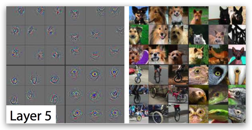
第五层
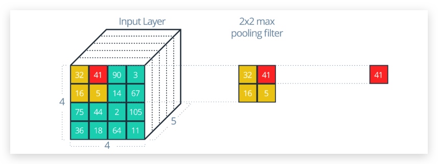
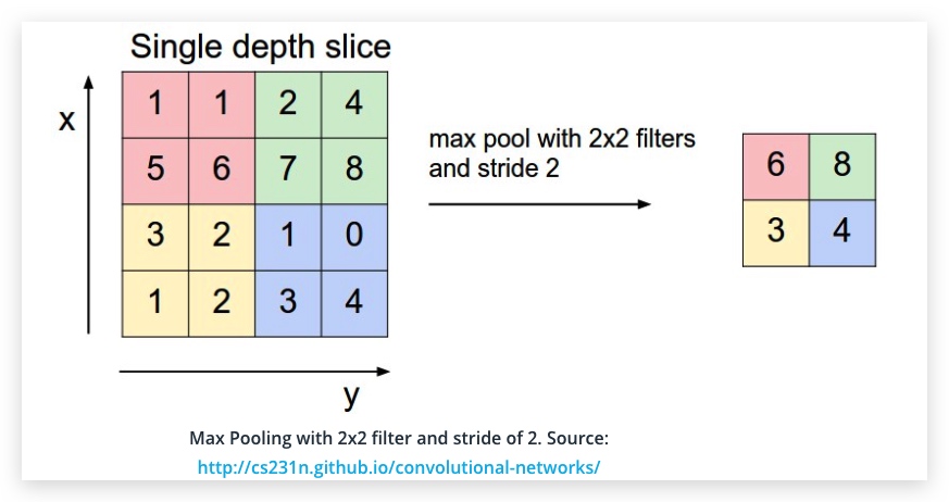
4. 池化
通过调整步长,我们可以降低图像的采样率,即移除一些图像信息,此外我们还可以将相邻的卷积进行聚合,得到一个卷积值来降低采样率,这个过程叫做池化。池化用来减少输出尺寸,避免过拟合。
- 最大池化
- 平均池化
最大池化的特点:
- 不会增加参数,不必担心过拟合
- 通常会提高模型准确率
- 计算量更大,因为步长小了
- 超参数增加:池区大小、池化步幅
将池区中的卷积去最大值保留
conv_layer = tf.nn.conv2d(input, weight, strides=[1, 2, 2, 1], padding='SAME')
conv_layer = tf.nn.bias_add(conv_layer, bias)
conv_layer = tf.nn.relu(conv_layer)
# Apply Max Pooling
conv_layer = tf.nn.max_pool(
    conv_layer,
    ksize=[1, 2, 2, 1],
    strides=[1, 2, 2, 1],
    padding='SAME')
The ksize and strides parameters are structured as 4-element lists, with each element corresponding to a dimension of the input tensor ([batch, height, width, channels]). For both ksize and strides, the batch and channel dimensions are typically set to 1.
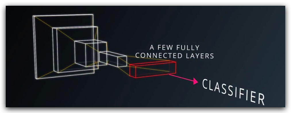
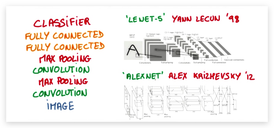
典型的CNN结构

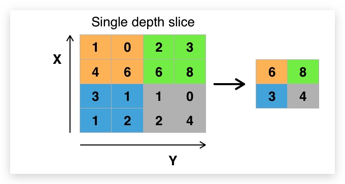
池化层的输出
池化层不改变输出的深度,它单独应用到每一个深度切片上。
假定:H = height, W = width, D = depth
- We have an input of shape 4x4x5 (HxWxD)
- Filter of shape 2x2 (HxW)
- A stride of 2 for both the height and width (S)
new_height = (input_height - filter_height)/S + 1
new_width = (input_width - filter_width)/S + 1
输出层的尺寸为2x2x5
input = tf.placeholder(tf.float32, (None, 4, 4, 5))
filter_shape = [1, 2, 2, 1]
strides = [1, 2, 2, 1]
padding = 'VALID'
pool = tf.nn.max_pool(input, filter_shape, strides, padding)
输出结果为 [1, 2, 2, 5], 即使padding方式修改为: 'SAME'
5. 1x1卷积
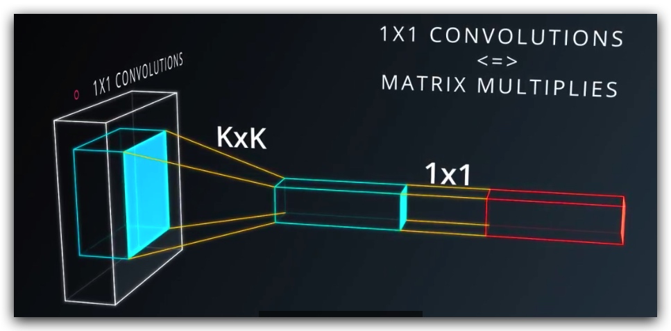
1x1卷积可以增加输出的深度,且运算非常简单
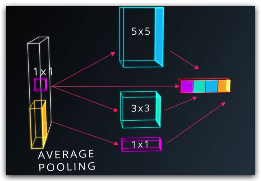
6. inception 模块
3. 使用Tensorflow构建CNN
TensorFlow 提供了 tf.nn.conv2d()和tf.nn.bias_add() 两个函数来构建CNN
# Output depth
k_output = 64

# Image Properties
image_width = 10
image_height = 10
color_channels = 3

# Convolution filter
filter_size_width = 5
filter_size_height = 5

# Input/Image
input = tf.placeholder(
    tf.float32,
    shape=[None, image_height, image_width, color_channels])

# Weight and bias
weight = tf.Variable(tf.truncated_normal(
    [filter_size_height, filter_size_width, color_channels, k_output]))
bias = tf.Variable(tf.zeros(k_output))

# Apply Convolution
conv_layer = tf.nn.conv2d(input, weight, strides=[1, 2, 2, 1], padding='SAME')
# Add bias
conv_layer = tf.nn.bias_add(conv_layer, bias)
# Apply activation function
conv_layer = tf.nn.relu(conv_layer)
使用 tf.nn.conv2d() 来构建一个卷积层,步长是**[1, 2, 2, 1],分别对应[batch, input_height, input_width, input_channels]**, 其中,batch和input_channels我们一般就设置为1。
例程
from tensorflow.examples.tutorials.mnist import input_data
mnist = input_data.read_data_sets(".", one_hot=True, reshape=False)

import tensorflow as tf

# Parameters
learning_rate = 0.00001
epochs = 10
batch_size = 128

# Number of samples to calculate validation and accuracy
# Decrease this if you're running out of memory to calculate accuracy
test_valid_size = 256

# Network Parameters
n_classes = 10  # MNIST total classes (0-9 digits)
dropout = 0.75  # Dropout, probability to keep units
# Store layers weight & bias
weights = {
    'wc1': tf.Variable(tf.random_normal([5, 5, 1, 32])),
    'wc2': tf.Variable(tf.random_normal([5, 5, 32, 64])),
    'wd1': tf.Variable(tf.random_normal([7*7*64, 1024])),
    'out': tf.Variable(tf.random_normal([1024, n_classes]))}

biases = {
    'bc1': tf.Variable(tf.random_normal([32])),
    'bc2': tf.Variable(tf.random_normal([64])),
    'bd1': tf.Variable(tf.random_normal([1024])),
    'out': tf.Variable(tf.random_normal([n_classes]))}
卷积
def conv2d(input):
    # Filter (weights and bias)
    F_W = tf.Variable(tf.truncated_normal((2, 2, 1, 3)))
    F_b = tf.Variable(tf.zeros(3))
    strides = [1, 2, 2, 1]
    padding = 'VALID'
    return tf.nn.conv2d(input, F_W, strides, padding) + F_b
最大池化
def maxpool2d(x, k=2):
    return tf.nn.max_pool(
        x,
        ksize=[1, k, k, 1],
        strides=[1, k, k, 1],
        padding='SAME')
模型结构
def conv_net(x, weights, biases, dropout):
    # Layer 1 - 28*28*1 to 14*14*32
    conv1 = conv2d(x, weights['wc1'], biases['bc1'])
    conv1 = maxpool2d(conv1, k=2)

    # Layer 2 - 14*14*32 to 7*7*64
    conv2 = conv2d(conv1, weights['wc2'], biases['bc2'])
    conv2 = maxpool2d(conv2, k=2)

    # Fully connected layer - 7*7*64 to 1024
    fc1 = tf.reshape(conv2, [-1, weights['wd1'].get_shape().as_list()[0]])
    fc1 = tf.add(tf.matmul(fc1, weights['wd1']), biases['bd1'])
    fc1 = tf.nn.relu(fc1)
    fc1 = tf.nn.dropout(fc1, dropout)

    # Output Layer - class prediction - 1024 to 10
    out = tf.add(tf.matmul(fc1, weights['out']), biases['out'])
    return out
Session
# tf Graph input
x = tf.placeholder(tf.float32, [None, 28, 28, 1])
y = tf.placeholder(tf.float32, [None, n_classes])
keep_prob = tf.placeholder(tf.float32)

# Model
logits = conv_net(x, weights, biases, keep_prob)

# Define loss and optimizer
cost = tf.reduce_mean(\
    tf.nn.softmax_cross_entropy_with_logits(logits=logits, labels=y))
optimizer = tf.train.GradientDescentOptimizer(learning_rate=learning_rate)\
    .minimize(cost)

# Accuracy
correct_pred = tf.equal(tf.argmax(logits, 1), tf.argmax(y, 1))
accuracy = tf.reduce_mean(tf.cast(correct_pred, tf.float32))

# Initializing the variables
init = tf. global_variables_initializer()

# Launch the graph
with tf.Session() as sess:
    sess.run(init)

    for epoch in range(epochs):
        for batch in range(mnist.train.num_examples//batch_size):
            batch_x, batch_y = mnist.train.next_batch(batch_size)
            sess.run(optimizer, feed_dict={
                x: batch_x,
                y: batch_y,
                keep_prob: dropout})

            # Calculate batch loss and accuracy
            loss = sess.run(cost, feed_dict={
                x: batch_x,
                y: batch_y,
                keep_prob: 1.})
            valid_acc = sess.run(accuracy, feed_dict={
                x: mnist.validation.images[:test_valid_size],
                y: mnist.validation.labels[:test_valid_size],
                keep_prob: 1.})

            print('Epoch {:>2}, Batch {:>3} -'
                  'Loss: {:>10.4f} Validation Accuracy: {:.6f}'.format(
                epoch + 1,
                batch + 1,
                loss,
                valid_acc))

    # Calculate Test Accuracy
    test_acc = sess.run(accuracy, feed_dict={
        x: mnist.test.images[:test_valid_size],
        y: mnist.test.labels[:test_valid_size],
        keep_prob: 1.})
    print('Testing Accuracy: {}'.format(test_acc))
4. 实现LeNet
预处理
An MNIST image is initially 784 features (1D). If the data is not normalized from [0, 255] to [0, 1], normalize it. We reshape this to (28, 28, 1) (3D), and pad the image with 0s such that the height and width are 32 (centers digit further). Thus, the input shape going into the first convolutional layer is 32x32x1.
网络模型规格
| 分层 | 输入 | 输出 | 备注 |
|---|---|---|---|
| 卷积层-1 | 32x32x1 | 28x28x6 | |
| 激活层-1 | 28x28x6 | 激活函数 | |
| 池化层-1 | 28x28x6 | 14x14x6 | 使用kernel大小为2,步长为2进行池化 |
| 卷积层-2 | 14x14x6 | 10x10x16 | 使用fliter 5*5 |
| 激活层-2 | 10x10x16 | 10x10x16 | |
| 池化层-2 | 10x10x16 | 5x5x16 | 使用kernel大小为2,步长为2进行池化 |
| 扁平层 | 5x5x16 | 转换为1维数据: 400 | tf.contrib.layers.flatten |
| 全连接层-1 | 400 | 120 | tf.Variable(tf.truncated_normal(shape=(400, 120), mean = mu, stddev = sigma)) |
| 激活层-3 | 120 | 120 | |
| 全连接层-2 | 120 | 84 | |
| 激活层-4 | 84 | 84 | |
| 全连接层-3 | 84 | 10 |
pipeline
rate = 0.001 #学习速率

logits = LeNet(x)
cross_entropy = tf.nn.softmax_cross_entropy_with_logits(labels=one_hot_y, logits=logits)
loss_operation = tf.reduce_mean(cross_entropy)
optimizer = tf.train.AdamOptimizer(learning_rate = rate)
training_operation = optimizer.minimize(loss_operation)
交叉熵函数:tf.nn.softmax_cross_entropy_with_logits
全局均值计算:tf.reduce_mean(cross_entropy)
优化函数:tf.train.AdamOptimizer 是改进的梯度下降法