深度神经网络
1. 深度神经网络简介
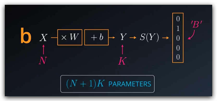
1. 线性模型复杂度
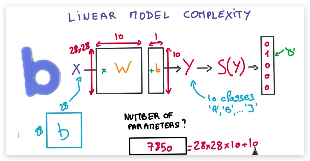
线性模型中,可调参数个数=w维数展开+b维数展开,即当我们有N个输入,K个输出时,我们的可调参数个数为(N+1)K
- 线性模型比较稳定,因为数据是线性叠加的,微小的输入不会引起结果的剧烈变化
- 因为模型是线性的,所以能够表示的关系是有限的,只能表示线性关系(输入是相加而非相乘)
- 线性函数的导数是常量
- 我们希望模型是非线性的,但是参数存放在线性的方程中,因此我们必须添加非线性成分
- 我们需要大量的可调参数,而不是固定的(N+1)K个
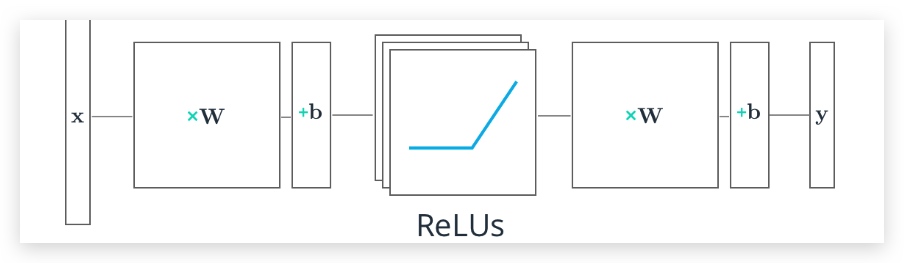
2. Rectified Linear Units(ReLUs)
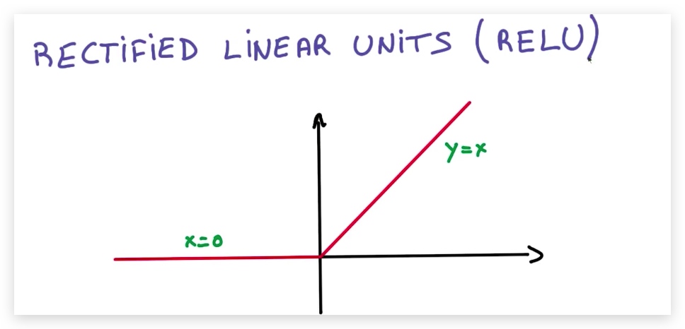
为了解决上一节提出的问题,我们引入ReLU函数,将其插入到矩阵中。以往,我们在构造多层的神经网络时,不同层的W是相乘的,然后得到一个W作为整体参与到结果的运算中,现在我们需要在Wi相乘的过程中插入ReLUs,这样模型就变成非线性模型来,同时我们可以调节隐藏层ReLUs的数量以达到增加参数的目的。
注意
ReLUs也是一种激活函数,目前我们已经接触到的激活函数有:sigmoid,softmax,ReLUs
在tensorflow中,我们使用tf.nn.relu()来调用relu函数
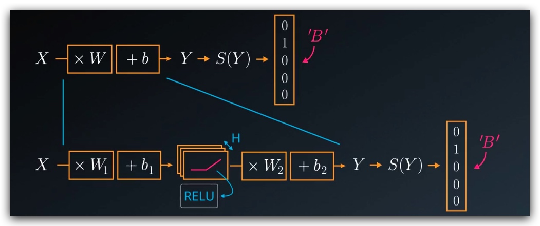
3. Multilayer Neural Networks
在网络中添加隐藏层可以让模型变得更复杂,同时,在隐藏层中添加非线性的激活函数,可以让模型变成非线性的。
假定我们构造一个2层的神经网络:
- 第一层保护来一组权重和偏差,我们将X输入到这一层,并传入到激活函数ReLUs中,输出的结果会输入到下一层(隐藏层)
- 隐藏层将结果和本层的权重、偏差进行计算,得到输出层结果y,然后使用softmax函数将其转换为概率
# Hidden Layer with ReLU activation function
hidden_layer = tf.add(tf.matmul(features, hidden_weights), hidden_biases)
hidden_layer = tf.nn.relu(hidden_layer)

output = tf.add(tf.matmul(hidden_layer, output_weights), output_biases)
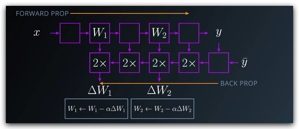
4. 链式法则及反向传播
这里我们同样会利用导数的链式法则,通过求解各部分导数,然后将其相乘,得到总体的导数。可以参考链式法则
2. 基于tensorflow的深度神经网络
1. 例程
学习参数
import tensorflow as tf

# Parameters
learning_rate = 0.001
training_epochs = 20
batch_size = 128  # Decrease batch size if you don't have enough memory
display_step = 1

n_input = 784  # MNIST data input (img shape: 28*28)
n_classes = 10  # MNIST total classes (0-9 digits)
隐藏层参数
n_hidden_layer = 256 # layer number of features
权重和偏差
这里我们为不同的层创建不同的权重和偏差
# Store layers weight & bias
weights = {
    'hidden_layer': tf.Variable(tf.random_normal([n_input, n_hidden_layer])),
    'out': tf.Variable(tf.random_normal([n_hidden_layer, n_classes]))
}
biases = {
    'hidden_layer': tf.Variable(tf.random_normal([n_hidden_layer])),
    'out': tf.Variable(tf.random_normal([n_classes]))
}
输入
# tf Graph input
x = tf.placeholder("float", [None, 28, 28, 1])
y = tf.placeholder("float", [None, n_classes])

x_flat = tf.reshape(x, [-1, n_input])
多层感知元
# Hidden layer with RELU activation
layer_1 = tf.add(tf.matmul(x_flat, weights['hidden_layer']),\
    biases['hidden_layer'])
layer_1 = tf.nn.relu(layer_1)
# Output layer with linear activation
logits = tf.add(tf.matmul(layer_1, weights['out']), biases['out'])
优化器
# Define loss and optimizer
cost = tf.reduce_mean(\
    tf.nn.softmax_cross_entropy_with_logits(logits=logits, labels=y))
optimizer = tf.train.GradientDescentOptimizer(learning_rate=learning_rate)\
    .minimize(cost)
会话
# Initializing the variables
init = tf.global_variables_initializer()


# Launch the graph
with tf.Session() as sess:
    sess.run(init)
    # Training cycle
    for epoch in range(training_epochs):
        total_batch = int(mnist.train.num_examples/batch_size)
        # Loop over all batches
        for i in range(total_batch):
            batch_x, batch_y = mnist.train.next_batch(batch_size)
            # Run optimization op (backprop) and cost op (to get loss value)
            sess.run(optimizer, feed_dict={x: batch_x, y: batch_y})
2. 训练神经网络
我们可以有两种方式来扩展我们的神经网络
- 更广:增加隐藏层H的数量,但是参数过多会难以训练
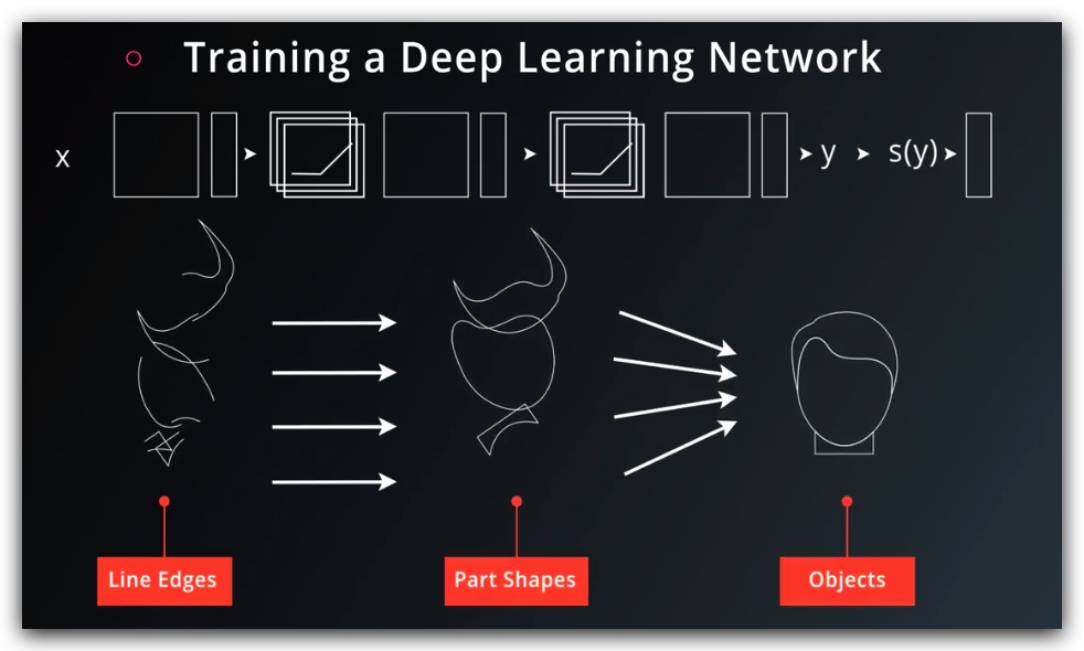
- 更深:增加多层神经网络
更深的方向是比较好的思路,一方面参数比较少,另一方面它会呈现出明显的结构特征,每一层可以学到不同的信息。学习速率也更快。
学习完成之后,我们自然希望将结果存储下来,此时可以使用:tf.train.Saver.
3. 储存变量和模型
储存变量
使用tf.train.Saver.save() 函数储存数据到**.ckpt格式文件中**. (checkpoint)
import tensorflow as tf

# The file path to save the data
save_file = './model.ckpt'

# Two Tensor Variables: weights and bias
weights = tf.Variable(tf.truncated_normal([2, 3]))
bias = tf.Variable(tf.truncated_normal([3]))

# Class used to save and/or restore Tensor Variables
saver = tf.train.Saver()

with tf.Session() as sess:
    # Initialize all the Variables
    sess.run(tf.global_variables_initializer())

    # Show the values of weights and bias
    print('Weights:')
    print(sess.run(weights))
    print('Bias:')
    print(sess.run(bias))

    # Save the model
    saver.save(sess, save_file)
加载数据
因为tf.train.Saver.restore()函数在载入时会设置数据,不必要再调用tf.global_variables_initializer().
# Remove the previous weights and bias
tf.reset_default_graph()

# Two Variables: weights and bias
weights = tf.Variable(tf.truncated_normal([2, 3]))
bias = tf.Variable(tf.truncated_normal([3]))

# Class used to save and/or restore Tensor Variables
saver = tf.train.Saver()

with tf.Session() as sess:
    # Load the weights and bias
    saver.restore(sess, save_file)

    # Show the values of weights and bias
    print('Weight:')
    print(sess.run(weights))
    print('Bias:')
    print(sess.run(bias))
储存完整模型
import math

save_file = './train_model.ckpt'
batch_size = 128
n_epochs = 100

saver = tf.train.Saver()

# Launch the graph
with tf.Session() as sess:
    sess.run(tf.global_variables_initializer())

    # Training cycle
    for epoch in range(n_epochs):
        total_batch = math.ceil(mnist.train.num_examples / batch_size)

        # Loop over all batches
        for i in range(total_batch):
            batch_features, batch_labels = mnist.train.next_batch(batch_size)
            sess.run(
                optimizer,
                feed_dict={features: batch_features, labels: batch_labels})

        # Print status for every 10 epochs
        if epoch % 10 == 0:
            valid_accuracy = sess.run(
                accuracy,
                feed_dict={
                    features: mnist.validation.images,
                    labels: mnist.validation.labels})
            print('Epoch {:<3} - Validation Accuracy: {}'.format(
                epoch,
                valid_accuracy))

    # Save the model
    saver.save(sess, save_file)
    print('Trained Model Saved.')
加载模型
saver = tf.train.Saver()

# Launch the graph
with tf.Session() as sess:
    saver.restore(sess, save_file)

    test_accuracy = sess.run(
        accuracy,
        feed_dict={features: mnist.test.images, labels: mnist.test.labels})

print('Test Accuracy: {}'.format(test_accuracy))
4. 加载参数到新的模型
TensorFlow 使用name参数来标记张量和运算,如果没有设置name,则tensorflow会自动设置为<Type>_<number>,根据变量声明的顺序和类型来命名。因此,如果将一个模型的参数导入另一个,可能会因为顺序等原因,造成错误的自动赋值,因此我们需要手工的指定。
import tensorflow as tf

tf.reset_default_graph()

save_file = 'model.ckpt'

# Two Tensor Variables: weights and bias
weights = tf.Variable(tf.truncated_normal([2, 3]), name='weights_0')
bias = tf.Variable(tf.truncated_normal([3]), name='bias_0')

saver = tf.train.Saver()

# Print the name of Weights and Bias
print('Save Weights: {}'.format(weights.name))
print('Save Bias: {}'.format(bias.name))

with tf.Session() as sess:
    sess.run(tf.global_variables_initializer())
    saver.save(sess, save_file)

# Remove the previous weights and bias
tf.reset_default_graph()

# Two Variables: weights and bias
bias = tf.Variable(tf.truncated_normal([3]), name='bias_0')
weights = tf.Variable(tf.truncated_normal([2, 3]) ,name='weights_0')

saver = tf.train.Saver()

# Print the name of Weights and Bias
print('Load Weights: {}'.format(weights.name))
print('Load Bias: {}'.format(bias.name))

with tf.Session() as sess:
    # Load the weights and bias - No Error
    saver.restore(sess, save_file)

print('Loaded Weights and Bias successfully.')
4. 正规化
「紧身裤」问题:紧身裤非常合身,但是难以穿上,因此我们会穿稍大一点的裤子。如果数据非常符合模型,将难以优化,因此我们会选择一个更泛化的模型,来防止出现过拟合。
防止过拟合的方法:
- 过早终止
- 正则化:对神经网络进行人为的约束,使得隐式的减少参数个数。
- L2
- dropout
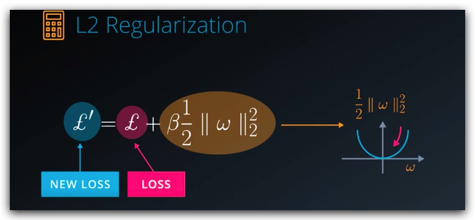
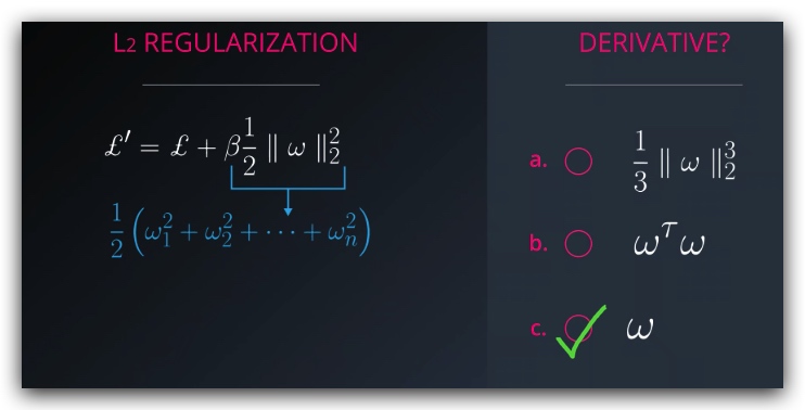
1. L2 正则化
L2 正则化非常简单,我们只需要在loss函数上加一部分,即所有向量的平方和/2,而不需要修改模型的结构,而且它的导数也非常的简单。
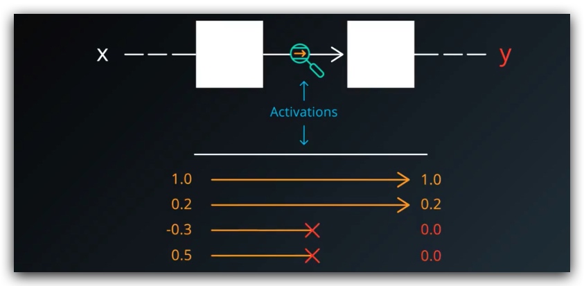
2. Dropout正则化
将训练的样本随机取一半设置为0,使的网络不依赖任何给定的激活存在,因为任何激活都可能被摧毁
 因此网络需要储存不同表示方法的冗余的数据
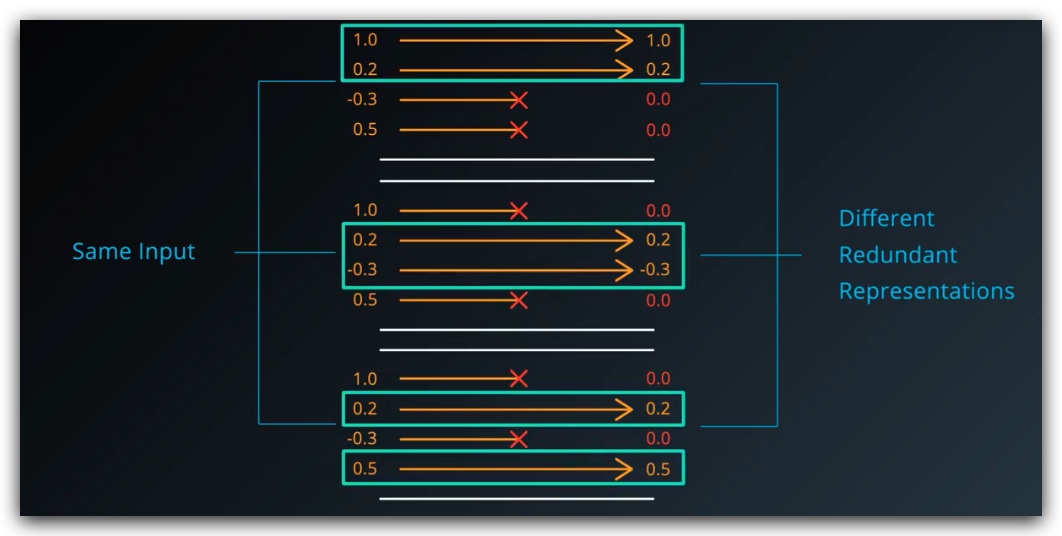 这种方法看上去有些啰嗦,实际上却可以增强网络的可靠性,并且能够防止过拟合
The tf.nn.dropout() function takes in two parameters:
hidden_layer: the tensor to which you would like to apply dropoutkeep_prob: the probability of keeping (i.e. not dropping) any given unit
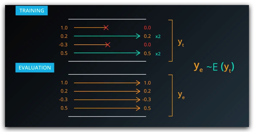
keep_prob allows you to adjust the number of units to drop. In order to compensate for dropped units, tf.nn.dropout() multiplies all units that are kept (i.e. not dropped) by 1/keep_prob.
During training, a good starting value for keep_prob is 0.5.
During testing, use a keep_prob value of 1.0 to keep all units and maximize the power of the model
扩展阅读