计算机视觉基础
1.车道线检测小程序
- 利用颜色进行检测
- 创建分割区域
- 边缘检测
- 直线提取
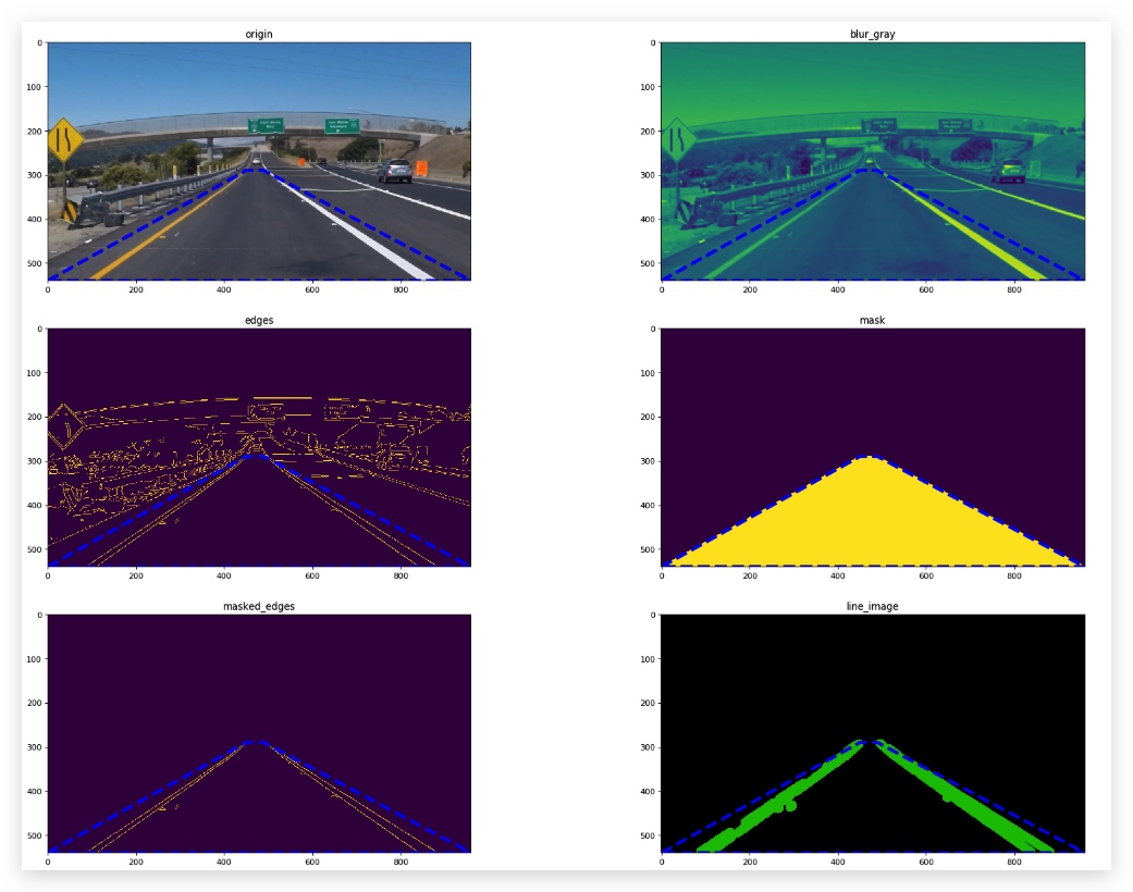
综合以上技术,尤其是2,3,4,我们可以对一些比较规则的图片进行检测,得到一个比较不错的车道线检测效果
import matplotlib.pyplot as plt
import matplotlib.image as mpimg
import numpy as np
import cv2
fig_size = 25
COL = 2
#绘图
def draw_imgs(imgs):
    fig = plt.figure(figsize=(fig_size,fig_size),dpi=80)
    for index,img in enumerate(imgs):
        plt.subplot(len(imgs)/COL+1, COL, index+1)
        #plt.imshow(img)
        plt.title(list(img.keys())[0])
        plt.imshow(list(img.values())[0])
        fig.tight_layout() #子图紧凑排版

#在每张图上绘制多边形
def draw_poly(vertices):
    x = []
    y = []
    for v in vertices:
        for xx,yy in v:
            x.append(xx)
            y.append(yy)
    x.append(x[0])
    y.append(y[0])
    plt.plot(x, y, 'b--', lw=4)
imgs = []
# Read in and grayscale the image
image = mpimg.imread('exit.jpg')
gray = cv2.cvtColor(image,cv2.COLOR_RGB2GRAY)

# Define a kernel size and apply Gaussian smoothing
###### 高斯模糊 #######
kernel_size = 5
blur_gray = cv2.GaussianBlur(gray,(kernel_size, kernel_size),0)

# Define our parameters for Canny and apply
###### canny 边缘检测 #######
low_threshold = 50
high_threshold = 150
edges = cv2.Canny(blur_gray, low_threshold, high_threshold)

# Next we'll create a masked edges image using cv2.fillPoly()
# 使用zeros_like构造一个和edges一样规模的零矩阵
mask = np.zeros_like(edges)
ignore_mask_color = 255

# This time we are defining a four sided polygon to mask
###### 构建多边形区域 #######
imshape = image.shape
vertices = np.array([[(0,imshape[0]),(450, 290), (490, 290), (imshape[1],imshape[0])]], dtype=np.int32)
cv2.fillPoly(mask, vertices, ignore_mask_color)
masked_edges = cv2.bitwise_and(edges, mask)


###### 霍夫变换检测直线段 #######
# Define the Hough transform parameters
# Make a blank the same size as our image to draw on
rho = 1 # distance resolution in pixels of the Hough grid
theta = np.pi/180 # angular resolution in radians of the Hough grid
threshold = 1     # minimum number of votes (intersections in Hough grid cell)
min_line_length = 5 #minimum number of pixels making up a line
max_line_gap = 1    # maximum gap in pixels between connectable line segments
line_image = np.copy(image)*0 # creating a blank to draw lines on

# Run Hough on edge detected image
# Output "lines" is an array containing endpoints of detected line segments
# 返回值是得到的霍夫变换检测到的符合条件的线段
lines = cv2.HoughLinesP(masked_edges, rho, theta, threshold, np.array([]),
                            min_line_length, max_line_gap)


# Iterate over the output "lines" and draw lines on a blank image
###### 给检测到到线段着色并绘制在图像上 #######
for line in lines:
    for x1,y1,x2,y2 in line:
        cv2.line(line_image,(x1,y1),(x2,y2),(0,200,0),20)

# Create a "color" binary image to combine with line image
color_edges = np.dstack((edges, edges, edges))

# Draw the lines on the edge image
lines_edges = cv2.addWeighted(color_edges, 0.8, line_image, 1, 0)

imgs.append({"origin":image})
imgs.append({"blur_gray":blur_gray})
imgs.append({"edges":edges})
imgs.append({"mask":mask})
imgs.append({"masked_edges":masked_edges})
imgs.append({"line_image":line_image}

draw_imgs(imgs,vertices)
2.相关库函数
1. numpy相关函数
| 功能 | 函数 | 使用 |
|---|---|---|
| 多边形拟合 | numpy.polyfit | |
| 深度方向叠加矩阵 | numpy.dstack |
2. matplotlib相关函数
| 功能 | 函数 | 使用 |
|---|---|---|
| 绘制子图 | matplotlib.pyplot..subplot | subplot(nrows, ncols, index, **kwargs) |
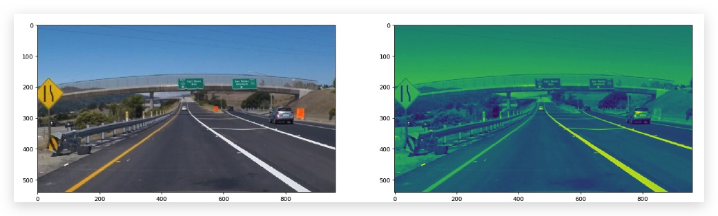
plt.figure(figsize=(fig_size,fig_size),dpi=80)
plt.subplot(1, 2, 1) # 一共绘制1行2列子图,这个是第1个
plt.imshow(image)
plt.subplot(1, 2, 2)# 一共绘制1行2列子图,这个是第2个
plt.imshow(gray)
https://blog.csdn.net/yuejisuo1948/article/details/81023125
3. opencv相关函数
| 功能 | 函数 | 用法 |
|---|---|---|
| 绘制线条 | cv2.line | cv2.line(img, pt1, pt2, color[, thickness[, lineType[, shift]]]) → img |
| 绘制多边形 | cv2.fillPoly | cv2.fillPoly(img, pts, color[, lineType[, shift[, offset]]]) → img |
| 按位与,即应用一个mask到目标图像 | cv2.bitwise_and | |
| 霍夫直线检测 | cv2.HoughLinesP |
cv2.inRange() for color selection cv2.fillPoly() for regions selection cv2.line() to draw lines on an image given endpoints cv2.addWeighted() to coadd / overlay two images cv2.cvtColor() to grayscale or change color cv2.imwrite() to output images to file cv2.bitwise_and() to apply a mask to an image
图片缩放
def save_image(filename,img):
    size = img.shape
    print(size)
    img2save = cv2.resize(img,(size[1]//2,size[0]//2),cv2.INTER_LINEAR)
    print(img2save.shape)
    plt.imsave("./examples/{0}.jpg".format(filename),img2save)
plot转换为图片
子图
def draw_poly(filename,img,vertices):
    fig = plt.figure()
    x = []
    y = []
    for v in vertices:
        for xx,yy in v:
            x.append(xx)
            y.append(yy)
            plt.plot(xx,yy,'.', color='red',markersize=20)
            note_point = "({0},{1})".format(xx,yy)
            plt.annotate(note_point,xy=(xx,yy),color='red')

    x.append(x[0])
    y.append(y[0])
    plt.plot(x, y, 'b--', lw=4)
    plt.imshow(img)
    #print(help(poly_img))
    fig.savefig("./examples/{0}.jpg".format(filename))
    #ax = plt.gca()
    #ax.invert_yaxis()
f, ((ax1, ax2) ,(ax3,ax4)) = plt.subplots(2, 2, figsize=(24, 9))
f.tight_layout()
ax1.imshow(image)
ax1.set_title('Original Image', fontsize=50)
ax3.imshow(grad_binary_x, cmap='gray')
ax3.set_title('Thresholded Gradient', fontsize=50)
plt.subplots_adjust(left=0., right=1, top=1.5, bottom=0.)
ax4.imshow(grad_binary_y, cmap='gray')
ax4.set_title('Thresholded Gradient', fontsize=50)
plt.subplots_adjust(left=0., right=1, top=1.5, bottom=0.)
dpi
3.图像矩阵及mask
4. 霍夫变换
1.霍夫变换
阅读材料2是一个非常好的了解霍夫变换的资料。在此做一些总结。
1. 斜率-截距空间
首先,我们在图像空间中,找到两个端点 (𝑥1,𝑦1) 和 (𝑥2,𝑦2),它们是可以构成一条直线的,但是我们先不去管通过它们的直线,但看每一个点,都有无限个直线,以不同的斜率m和截距b,通过这个点。
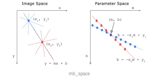
我们把y=mx+b变换成b=y-mx之后,实际上可以将这某个直线变换到一个以b和m做参数的空间中,此时,图像空间中的一条固定直线,因其b和m是定值,所以在m-b空间中是一个点(m,b)。 类似的,图像空间中的某个点(𝑥1,𝑦1) ,因其b和m符合b=y-mx方程,因此在m-b空间中是一条直线。
这时我们再看之前穿过 (𝑥1,𝑦1) 和 (𝑥2,𝑦2)的直线,这条直线上的所有的点,其斜率和截距都是m和b,因此这个直线上的所有的点,在m-b空间中都经过点(m,b)。
每当我们找到端点为 (𝑥1,𝑦1) 和 (𝑥2,𝑦2)的一条直线上的点,mb空间中的点(m,b)就会被一条直线经过,这个过程称为vote,因此,vote越多,说明我们在 (𝑥1,𝑦1) 和 (𝑥2,𝑦2)上找到的线段越多,越可能是直线。
2. 极坐标空间
上述m-b空间最大的问题是,截距可能会是无穷,这样在m-b空间上就找不到点(m,b)了。
因此引入极坐标空间。
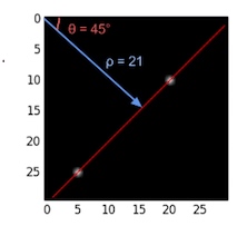
ρ = x cos θ + y sin θ

where:
ρ (rho) = distance from origin to the line. [-max_dist to max_dist].
          max_dist is the diagonal length of the image.
θ = angle from origin to the line. [-90° to 90°]
变换到霍夫空间中的时候,原图像中的点,变换为曲线,原图像中的直线,变换为点。因此两条曲线的焦点就表示找到了过这两个点的一条直线。
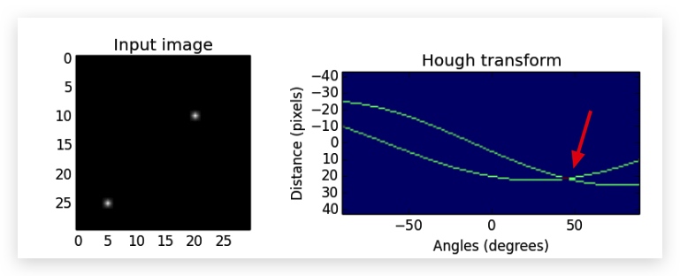
同样,越多的直线经过这两点,霍夫空间中的曲线焦点被相交的次数越多,vote次数也越多。
我们在实际的运用中,可以设定一个阈值,相交点被vote的次数为5,也就是说,在图像空间两个端点 (𝑥1,𝑦1) 和 (𝑥2,𝑦2),连成的直线上,我们至少还能找到其他5个点组成的线段。
rho = 1 # distance resolution in pixels of the Hough grid
theta = np.pi/180 # angular resolution in radians of the Hough grid
threshold = 100   #这个值越大,被检测到的直线段越少,有可能检测不到
min_line_len = 50 #minimum number of pixels making up a line
max_line_gap = 100    # maximum gap in pixels between connectable line segments
line_img,lines = hough_lines(masked_edges, rho, theta, threshold, min_line_len, max_line_gap)
TODO
绘图描述
5. 边缘检测之Canny
https://blog.csdn.net/wishchin/article/details/50969322
阅读材料