深度学习库——Tensorflow

关于 TensorFlow

TensorFlow™ 是一个采用数据流图（data flow graphs），用于数值计算的开源软件库。节点（Nodes）在图中表示数学操作，图中的线（edges）则表示在节点间相互联系的多维数据数组，即张量（tensor）。它灵活的架构让你可以在多种平台上展开计算，例如台式计算机中的一个或多个CPU（或GPU），服务器，移动设备等等。TensorFlow 最初由Google大脑小组（隶属于Google机器智能研究机构）的研究员和工程师们开发出来，用于机器学习和深度神经网络方面的研究，但这个系统的通用性使其也可广泛用于其他计算领域。

tensors_flowing

基础

Hello, Tensor World!

基本使用

使用 TensorFlow, 你必须明白 TensorFlow:

使用图 (graph) 来表示计算任务.
在被称之为会话 (Session) 的上下文 (context) 中执行图.
使用 tensor 表示数据.
通过变量 (Variable) 维护状态.
使用 feed 和 fetch 可以为任意的操作(arbitrary operation) 赋值或者从其中获取数据.

1. tf.constant 常量和session

import tensorflow as tf

# Create TensorFlow object called tensor
hello_constant = tf.constant('Hello World!')

with tf.Session() as sess:
    # Run the tf.constant operation in the session
    output = sess.run(hello_constant)
    print(output)

2. 输入

使用tf.placeholder()创建一个占位符，然后使用tf.session.run()中到feed_dict 参数将数据传入

import tensorflow as tf

output = None
x = tf.placeholder(tf.int32)

with tf.Session() as sess:
    output = sess.run(x,feed_dict = {x:12})
    print(output)

3. 数学运算

x = tf.add(5, 2)  # 7
x = tf.subtract(10, 4) # 6
y = tf.multiply(2, 5)  # 10
z = tf.divide(10,2) # 5

4. 类型转换

tf.subtract(tf.cast(tf.constant(2.0), tf.int32), tf.constant(1))   # 1

5. tf.Variable()

x = tf.Variable(5)

Training Your Classifier

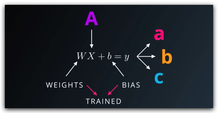
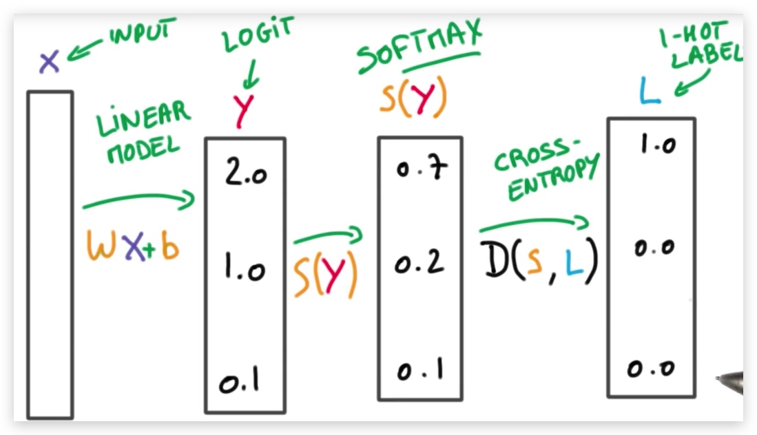
首先我们会训练模型，以确定权重W和偏差b的取值，然后利用W和b求解预测值y(logit)
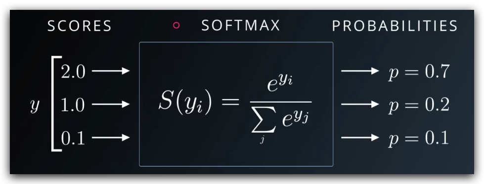
然后，使用softmax函数，将预测值y转换成对应的概率p

扩展阅读

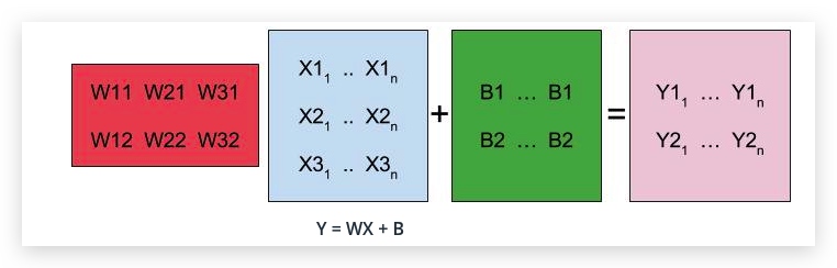
1. TensorFlow 线性方程

tf.global_variables_initializer()
tf.truncated_normal()

# Quiz Solution
import tensorflow as tf
def get_weights(n_features, n_labels):
    return tf.Variable(tf.truncated_normal((n_features, n_labels)))

def get_biases(n_labels):
    return tf.Variable(tf.zeros(n_labels))

def linear(input, w, b):
    return tf.add(tf.matmul(input, w), b)

2. Softmax

def softmax(x):
    """Compute softmax values for each sets of scores in x."""
    return np.exp(x) / np.sum(np.exp(x), axis=0)

logits = [3.0, 1.0, 0.2]
print(softmax(logits))

x = tf.nn.softmax([2.0, 1.0, 0.2])

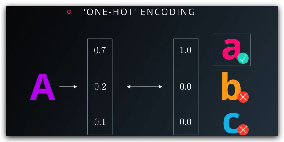
3. one-hot encoding

4. 交叉熵

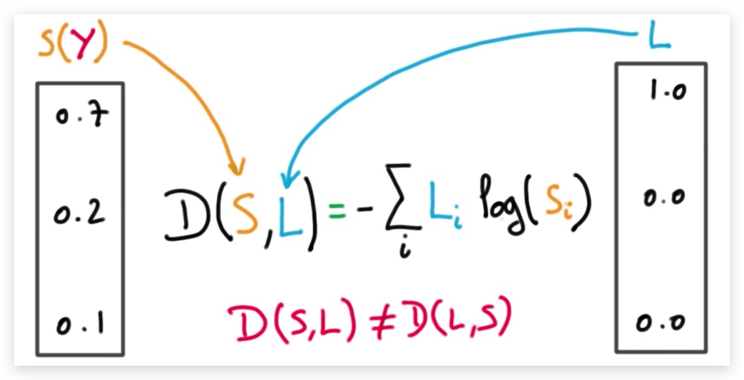
求logits和对应label的交叉熵，表示误差值。

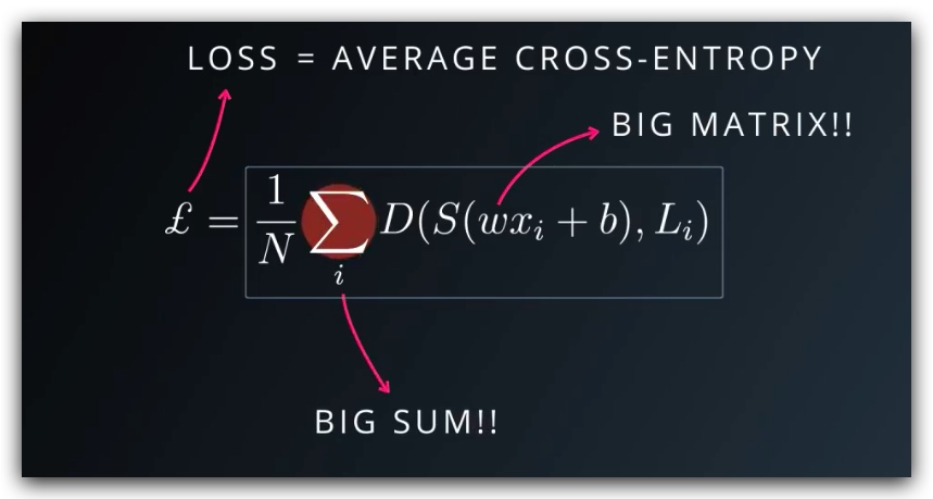我们通过训练来找到w和b，在这个过程中，我们需要不断缩小loss，即使用梯度下降的方法，缩小误差函数（交叉熵）

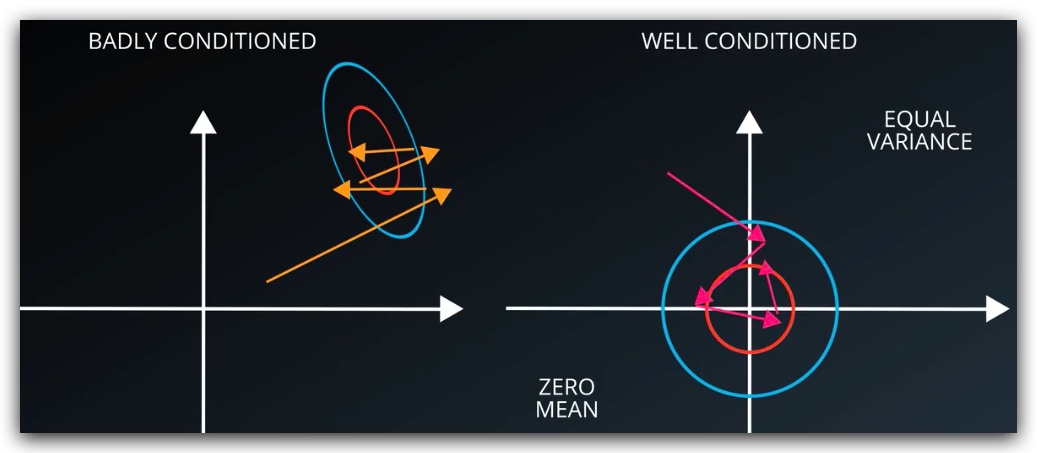
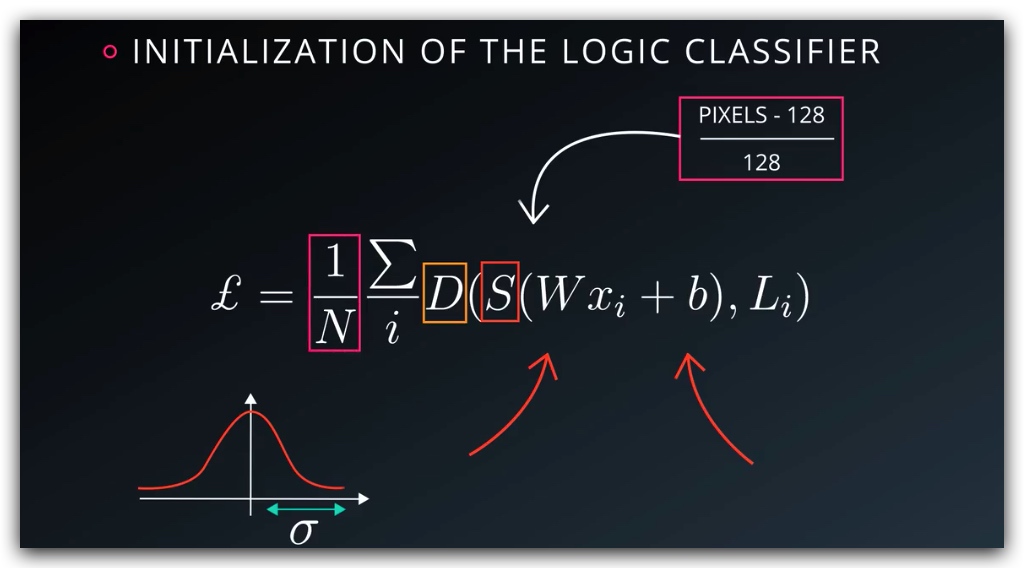
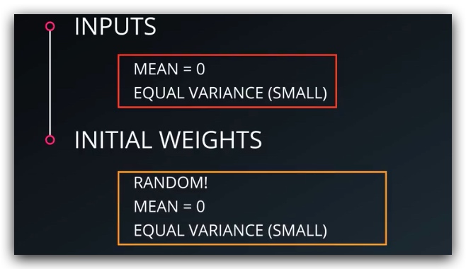
5. 归一化输入及初始权重

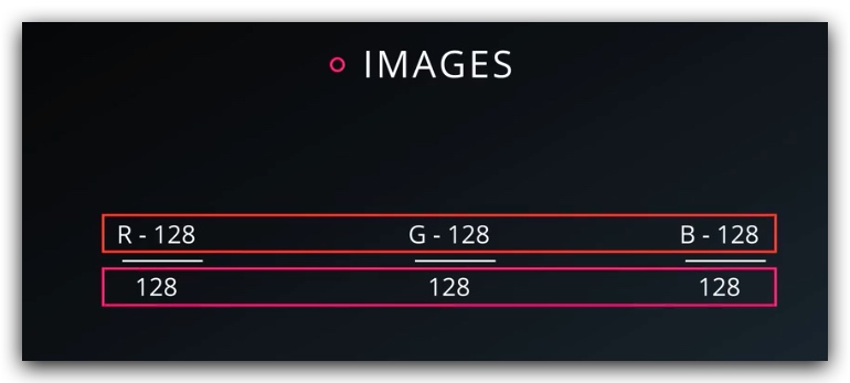
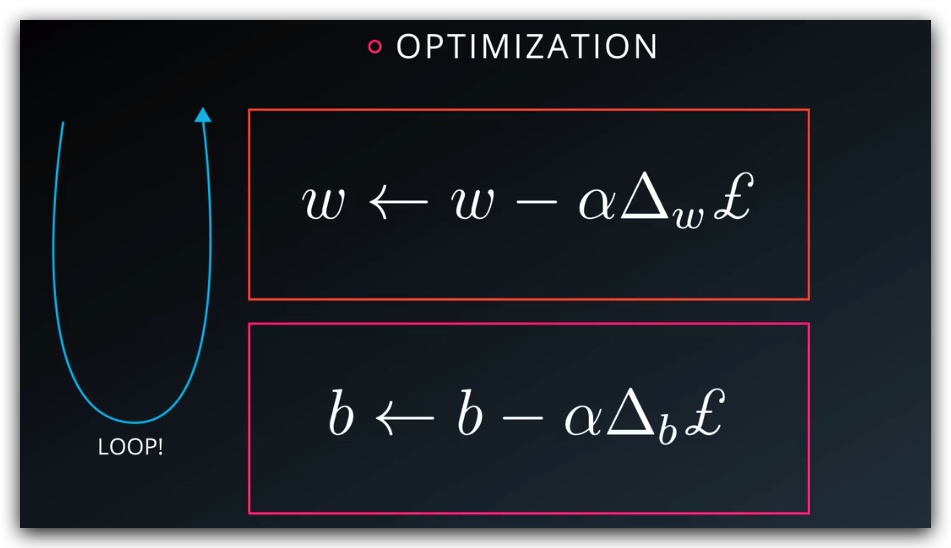
输入的变量为了便于优化器工作，要尽可能保证均值为0，且方差不变。 ) 对于图像来讲，可以使用下面的方法处理输入的每个像素。 $ X'=a+{\frac {\left(X-X_{\min }\right)\left(b-a\right)}{X_{\max }-X_{\min }}} $ 对于权重和偏差，最好从正态分布中取值，也要保证均值相同，方差不变（尽量小一些的sigma）反向求导，进行优化

6. 性能度量

训练数据集
验证数据集
测试数据集

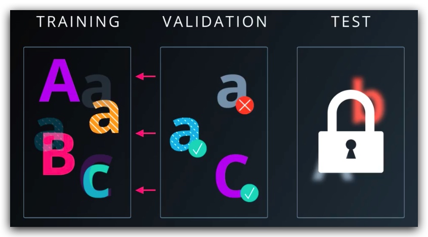
必须要单独隔离一部分的test数据，因为在调参过程中，我们会无意识的泄露验证集中的信息，导致测试数据不准确。

对于验证数据集和测试集的大小，自然是越大越好，当你调整的参数，使的有至少30个结果较之前有了变化，在统计学上才是有意义的。如果你有3000个数据，那么准确率必须提高或者降低0.1%，才是有意义的变化。因此一般来讲，我们需要至少30000个数据，来保证0.1%的精度。

此外，如果数据不均衡，例如某种类型的数据比例失衡，则不能使用该方法，我们需要增大数据集。比如使用交叉验证或直接获取数据

7. 随机梯度下降法（SGD）

求解loss函数的导数，大约是求解loss的三倍计算量，当数据集很大时，运算量会变的很大。因此我们需要一个办法来减少运算量，此处使用一种相对比较简单的方法，随机梯度下降。

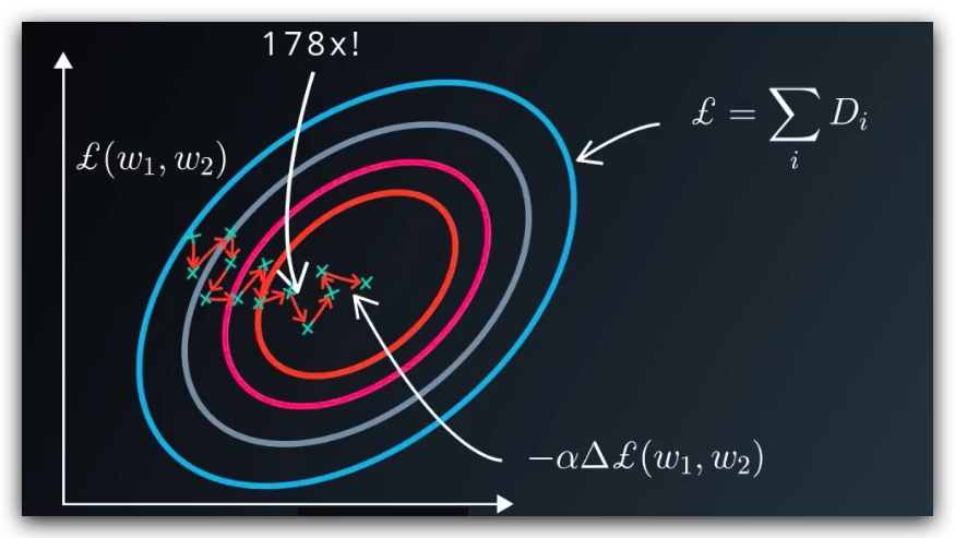
我们取一小部分的数据，计算它的导数，假定它时按照梯度下降的方向进行的，然后用它对参数进行更新（有时并不是下降），当随机次数足够多时，我们可以得到正确的结果。这种方法效率较高，但是有比较多的限制：

输入和权重初始值要遵循均值为0，方差不变且较小的要求
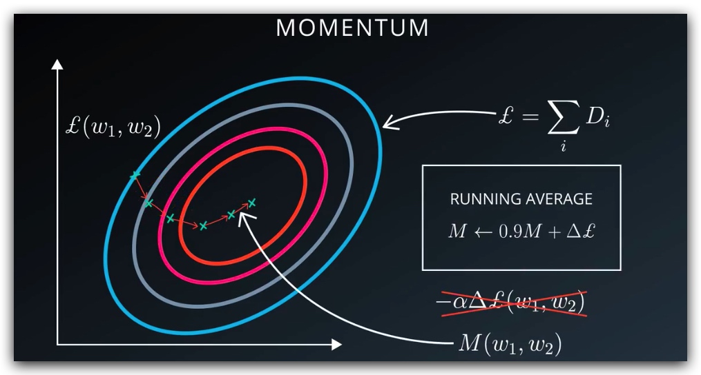
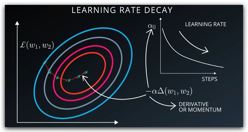
使用动量方法：使用梯度的实时平均值来更新权重，通常具有很好的收敛性
学习速率衰减：SGD可以有很多参数供我们调节，但是如果效果不好，请优先选择降低学习速率

8. Mini-batch 和 Epochs

我们可以取数据的子集来进行训练，称为batch，每次向模型输入batch_size大小的数据集
对我们的数据集进行一次feedforward和backforward，称之为一次Epochs。这个过程被用来不断提高模型的准确率。
通过调整batch_size（小）、Epochs（多）和learn_rate（低）可以得到较好的准确率

from tensorflow.examples.tutorials.mnist import input_data
import tensorflow as tf
import numpy as np
from helper import batches  # Helper function created in Mini-batching section


def print_epoch_stats(epoch_i, sess, last_features, last_labels):
    """
    Print cost and validation accuracy of an epoch
    """
    current_cost = sess.run(
        cost,
        feed_dict={features: last_features, labels: last_labels})
    valid_accuracy = sess.run(
        accuracy,
        feed_dict={features: valid_features, labels: valid_labels})
    print('Epoch: {:<4} - Cost: {:<8.3} Valid Accuracy: {:<5.3}'.format(
        epoch_i,
        current_cost,
        valid_accuracy))

n_input = 784  # MNIST data input (img shape: 28*28)
n_classes = 10  # MNIST total classes (0-9 digits)

# Import MNIST data
mnist = input_data.read_data_sets('/datasets/ud730/mnist', one_hot=True)

# The features are already scaled and the data is shuffled
train_features = mnist.train.images
valid_features = mnist.validation.images
test_features = mnist.test.images

train_labels = mnist.train.labels.astype(np.float32)
valid_labels = mnist.validation.labels.astype(np.float32)
test_labels = mnist.test.labels.astype(np.float32)

# Features and Labels
features = tf.placeholder(tf.float32, [None, n_input])
labels = tf.placeholder(tf.float32, [None, n_classes])

# Weights & bias
weights = tf.Variable(tf.random_normal([n_input, n_classes]))
bias = tf.Variable(tf.random_normal([n_classes]))

# Logits - xW + b
logits = tf.add(tf.matmul(features, weights), bias)

# Define loss and optimizer
learning_rate = tf.placeholder(tf.float32)
cost = tf.reduce_mean(tf.nn.softmax_cross_entropy_with_logits(logits=logits, labels=labels))
optimizer = tf.train.GradientDescentOptimizer(learning_rate=learning_rate).minimize(cost)

# Calculate accuracy
correct_prediction = tf.equal(tf.argmax(logits, 1), tf.argmax(labels, 1))
accuracy = tf.reduce_mean(tf.cast(correct_prediction, tf.float32))

init = tf.global_variables_initializer()

batch_size = 128
epochs = 10
learn_rate = 0.001

train_batches = batches(batch_size, train_features, train_labels)

with tf.Session() as sess:
    sess.run(init)

    # Training cycle
    for epoch_i in range(epochs):

        # Loop over all batches
        for batch_features, batch_labels in train_batches:
            train_feed_dict = {
                features: batch_features,
                labels: batch_labels,
                learning_rate: learn_rate}
            sess.run(optimizer, feed_dict=train_feed_dict)

        # Print cost and validation accuracy of an epoch
        print_epoch_stats(epoch_i, sess, batch_features, batch_labels)

    # Calculate accuracy for test dataset
    test_accuracy = sess.run(
        accuracy,
        feed_dict={features: test_features, labels: test_labels})

print('Test Accuracy: {}'.format(test_accuracy))

9. Session

correct_prediction = tf.equal(tf.argmax(logits, 1), tf.argmax(one_hot_y, 1))
accuracy_operation = tf.reduce_mean(tf.cast(correct_prediction, tf.float32))
saver = tf.train.Saver()

def evaluate(X_data, y_data):
    num_examples = len(X_data)
    total_accuracy = 0
    sess = tf.get_default_session()
    for offset in range(0, num_examples, BATCH_SIZE):
        batch_x, batch_y = X_data[offset:offset+BATCH_SIZE], y_data[offset:offset+BATCH_SIZE]
        accuracy = sess.run(accuracy_operation, feed_dict={x: batch_x, y: batch_y, keep_prob: 1.0})
        total_accuracy += (accuracy * len(batch_x))
    return total_accuracy / num_examples

session.run()来启动一次运算，

# 深度学习库——Tensorflow

# 关于 TensorFlow

# 基础

# Hello, Tensor World!

#基本使用

# 1. tf.constant 常量和session

# 2. 输入

# 3. 数学运算

# 4. 类型转换

# 5. tf.Variable()

# Training Your Classifier

# 1. TensorFlow 线性方程

# 2. Softmax

# 3. one-hot encoding

# 4. 交叉熵

# 5. 归一化输入及初始权重

# 6. 性能度量

# 7. 随机梯度下降法（SGD）

# 8. Mini-batch 和 Epochs

# 9. Session