Writeup

Advanced Lane Finding Project

The goals/steps of this project are the following:

Compute the camera calibration matrix and distortion coefficients given a set of chessboard images.
Apply a distortion correction to raw images.
Use color transforms, gradients, etc., to create a thresholded binary image.
Apply a perspective transform to rectify binary image ("birds-eye view").
Detect lane pixels and fit to find the lane boundary.
Determine the curvature of the lane and vehicle position with respect to the center.
Warp the detected lane boundaries back onto the original image.
Output visual display of the lane boundaries and numerical estimation of lane curvature and vehicle position.

Here I will consider the rubric points individually and describe how I addressed each point in my implementation.

the implementation can be found here

Camera Calibration

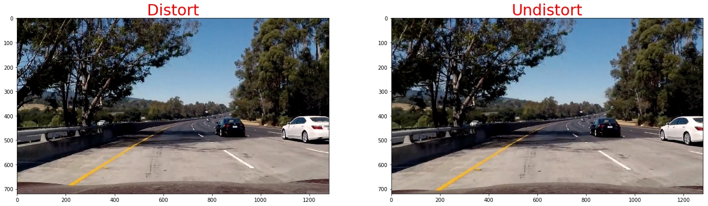
1. Briefly state how you computed the camera matrix and distortion coefficients. Provide an example of a distortion-corrected calibration image.

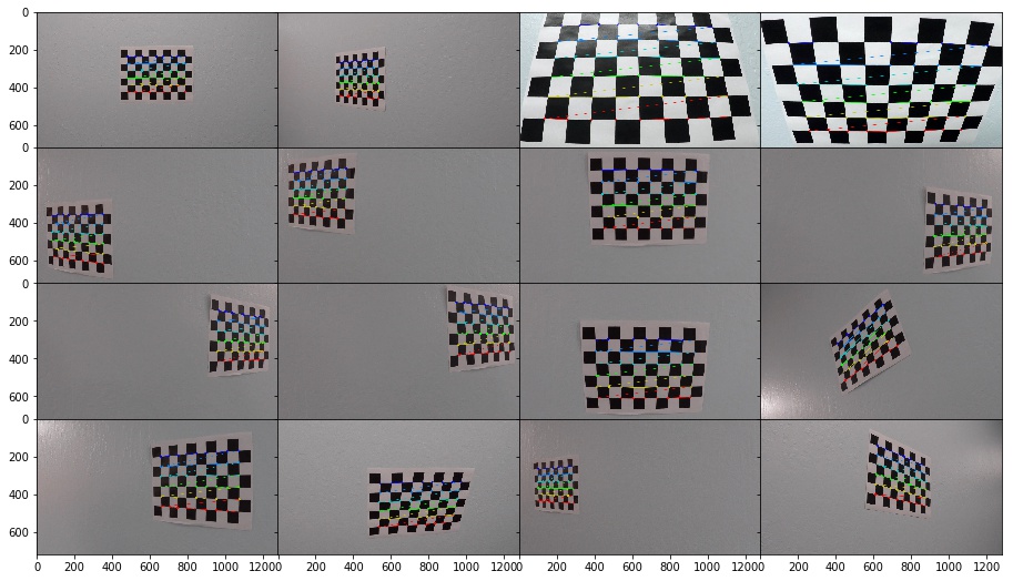
1. Prepared the object points and image points

The object points is the (x,y,z) corrdinates of the chessboard corners in the real world.By assuming the chessboard is fixed on the z plane(z=0).Thus the objp is as below:

# prepare object points, like (0,0,0), (1,0,0), (2,0,0) ....,(6,5,0)
objp = np.zeros((6*9,3), np.float32)
objp[:,:2] = np.mgrid[0:9,0:6].T.reshape(-1,2)

The image points is the corners we detected in the chessboard image as below:

ret, corners = cv2.findChessboardCorners(gray, (9,6),None)
if ret == True:
            objpoints.append(objp)
            imgpoints.append(corners)
            # Draw and display the corners
            annotated_images.append(cv2.drawChessboardCorners(img, (9,6), corners, ret))

2. Using those two points sets to calibrate camera:

ret, mtx, dist, rvecs, tvecs = cv2.calibrateCamera(objpoints, imgpoints, gray.shape[::-1], None, None)

draw_corners

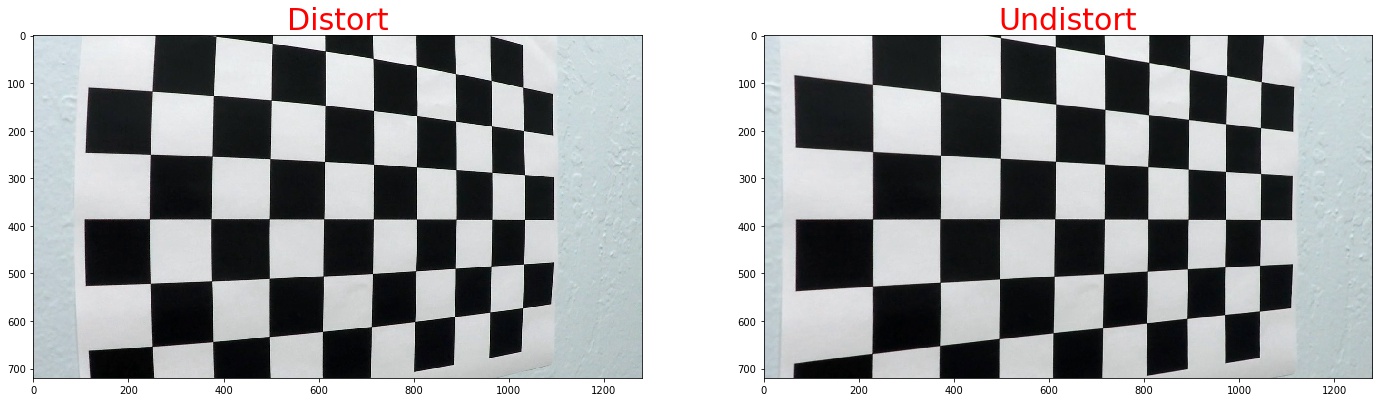
3. Using the `cv2.calibrateCamera` return to `undistort()` the image

def get_undistort_img(img,mtx,dist):
        return cv2.undistort(img, mtx, dist, None, mtx)

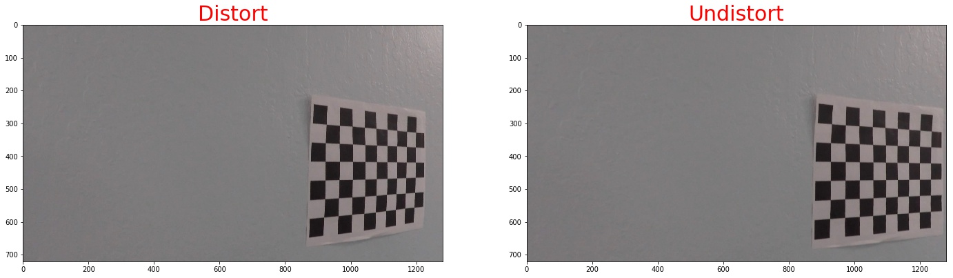
Undistort_calibration15 Undistort_calibration5

4. Then we apply the measurement to our test images

here I will show you some of the iamges Undistort_straight_lines1 Undistort_test3 Undistort_test5

Pipeline (single images)

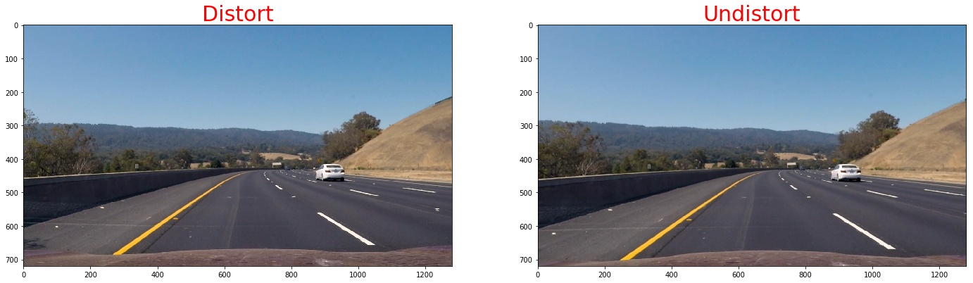
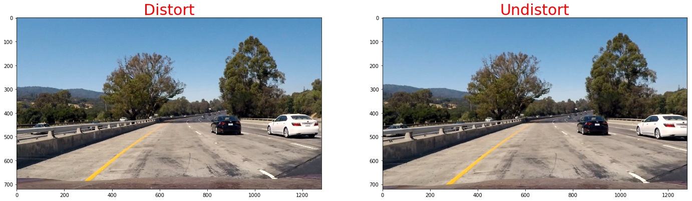
1. Provide an example of a distortion-corrected image.

To demonstrate this step, I will describe how I apply the distortion correction to one of the test images like this one:./imgs Undistort_straight_lines1

2. Describe how (and identify where in your code) you used color transforms, gradients or other methods to create a thresholded binary image. Provide an example of a binary image result.

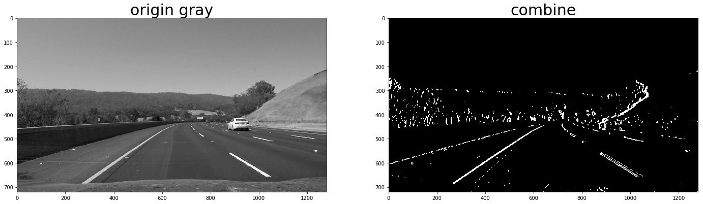
I used a combination of color and gradient thresholds to generate a binary image. Here's an example of my output for this step. (note: this is not actually from one of the test images)

Undistort_test1

1. We use sobel operator the take the gradient thresholds

Calculate the derivative in the xx direction (the 1, 0 at the end denotes xx direction):
sobelx = cv2.Sobel(gray, cv2.CV_64F, 1, 0)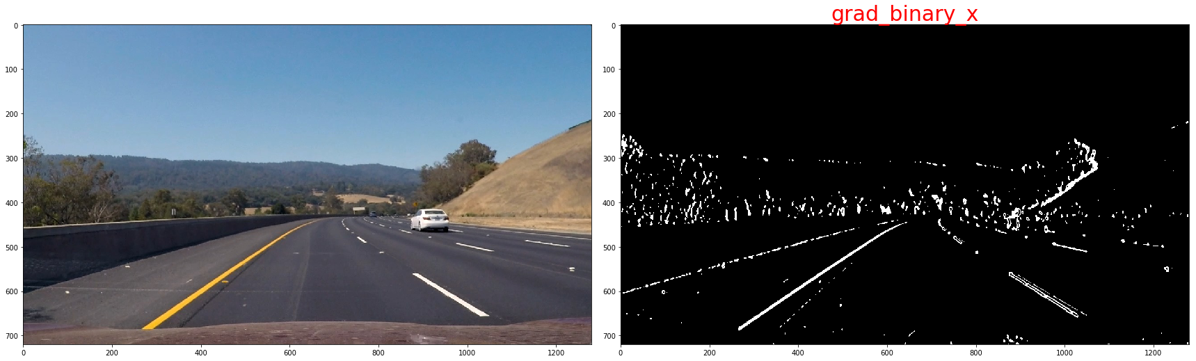
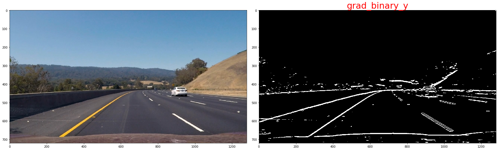
grad_binary_x Calculate the derivative in the yy direction (the 0, 1 at the end denotes yy direction): sobely = cv2.Sobel(gray, cv2.CV_64F, 0, 1)
Taking the gradient in the xx direction emphasizes edges closer to vertical. Alternatively, taking the gradient in the yy direction emphasizes edges closer to horizontal. grad_binary_y The magnitude, or absolute value, of the gradient is just the square root of the squares of the individual x and y gradients. For a gradient in both the xx and yy directions, the magnitude is the square root of the sum of the squares.

sobel_xy = np.sqrt(sobel_x**2 + sobel_y**2)
scaled_xy = np.uint8(255 * sobel_xy / np.max(sobel_xy))

mag_binary_xy

In the case of lane lines, we're interested only in edges of a particular orientation. So now we will explore the direction, or orientation, of the gradient.

sx_abs = np.absolute(cv2.Sobel(img, cv2.CV_64F, 1, 0, ksize=kernel_size))
sy_abs = np.absolute(cv2.Sobel(img, cv2.CV_64F, 0, 1, ksize=kernel_size))    
dir_sxy = np.arctan2(sx_abs, sy_abs)

dir_sobel_xy

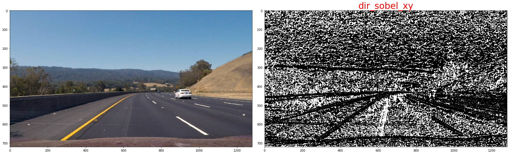
the threshold we use is as below:

	lower	upper
sobel-x	20	120
sobel-y	20	120
Magnitude of the Gradient	80	200
Direction of the Gradient	np.pi/4	np.pi/2

now,we will combine them to get a batter result, since the sobel-x will detect line close vertical,we'll keep it all

def combined_sobels(sx_binary, sy_binary, sxy_magnitude_binary,sxy_direction_binary):    
    combined = np.zeros_like(sxy_direction_binary)
    combined[(sx_binary == 1) | ((sy_binary == 1) & (sxy_magnitude_binary == 1) & (sxy_direction_binary == 1))] = 1
    return combined

combine

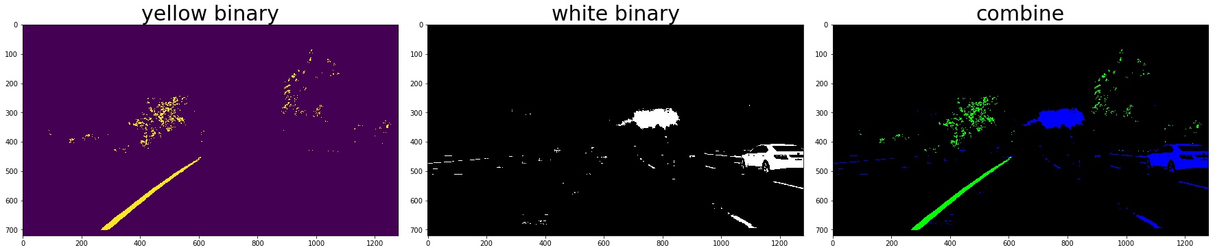
2. Color Thresholding

yellow_binary[((h >= 15) & (h <= 35))
                 & ((l >= 30) & (l <= 204))
                 & ((s >= 115) & (s <= 255))] = 1
white_binary = np.zeros_like(h)
white_binary[((h>= 0) & (h <= 255))
                 & ((l>= 200) & (l <= 255))
                 & ((s>= 0) & (s <= 255))] = 1

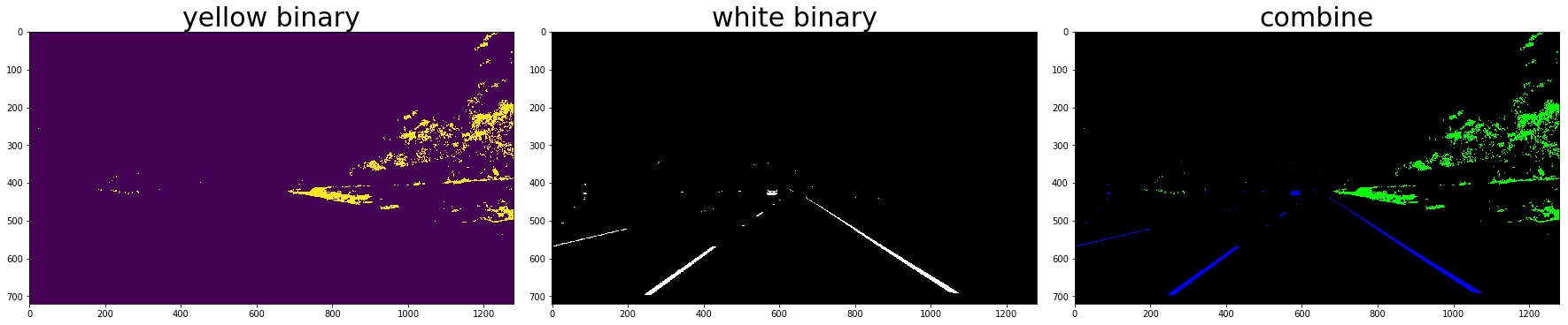
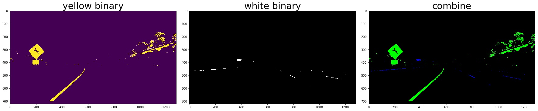
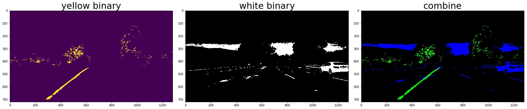
3. Combine the gradient and color threshed

color_binary_combined = np.dstack((combined_grad, combined_yellow_white, np.zeros_like(combined_grad))) * 255
combined_binary = np.zeros_like(gray)
combined_binary[(combined_grad == 1)|(combined_yellow_white == 1)] = 1

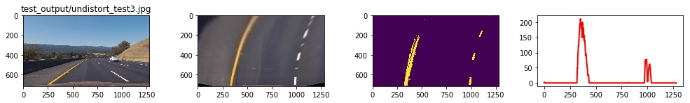
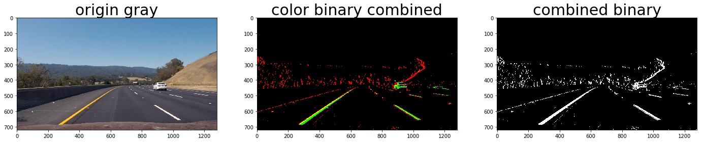combine_grad_colo the red line is detected by gradient and the green is detected by color

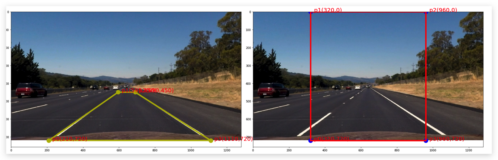
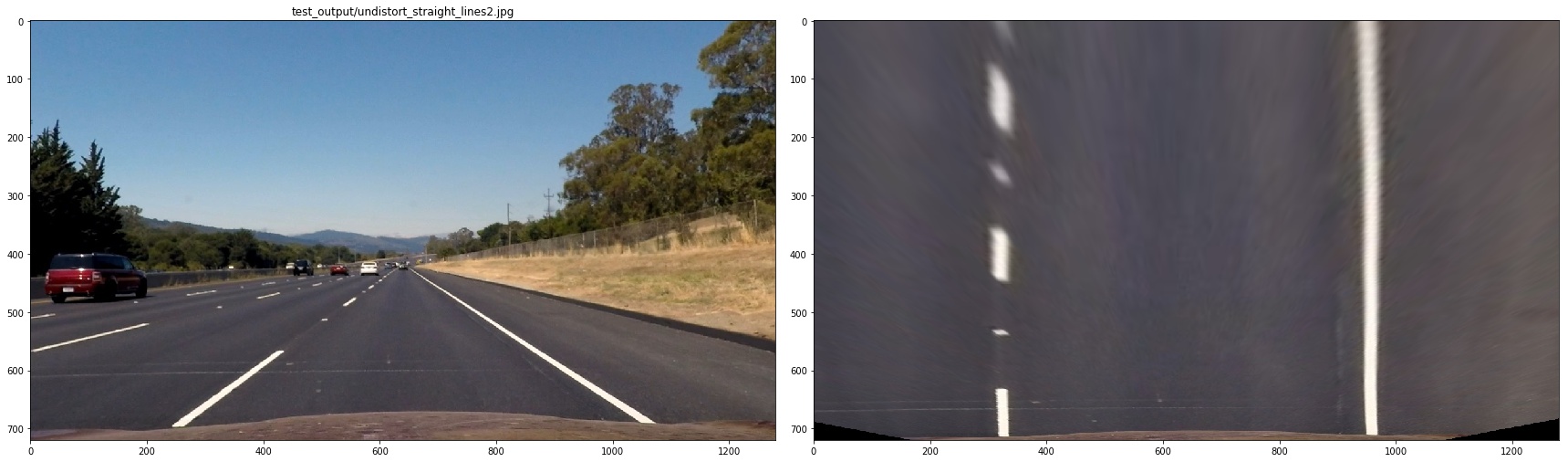
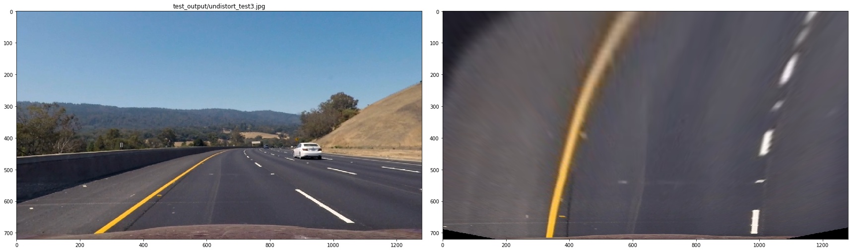
3. Describe how (and identify where in your code) you performed a perspective transform and provide an example of a transformed image.

The code for my perspective transform includes a function called warper(), which appears in lines 1 through 8 in the file example.py (./imgs/examples/example.py) (or, for example, in the 3rd code cell of the IPython notebook). The warper() function takes as inputs an image (img), as well as source (src) and destination (dst) points. I chose the hardcode the source and destination points in the following manner:

src = np.float32(
    [[(img_size[0] / 2) - 55, img_size[1] / 2 + 100],
    [((img_size[0] / 6) - 10), img_size[1]],
    [(img_size[0] * 5 / 6) + 60, img_size[1]],
    [(img_size[0] / 2 + 55), img_size[1] / 2 + 100]])
dst = np.float32(
    [[(img_size[0] / 4), 0],
    [(img_size[0] / 4), img_size[1]],
    [(img_size[0] * 3 / 4), img_size[1]],
    [(img_size[0] * 3 / 4), 0]])

note:the points should be clock-wise and start from the left-bottom, the src and the des should have the same orders otherwise the result picture will be upside down or twisted.

bird_view_trans

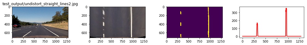
4. Describe how (and identify where in your code) you identified lane-line pixels and fit their positions with a polynomial?

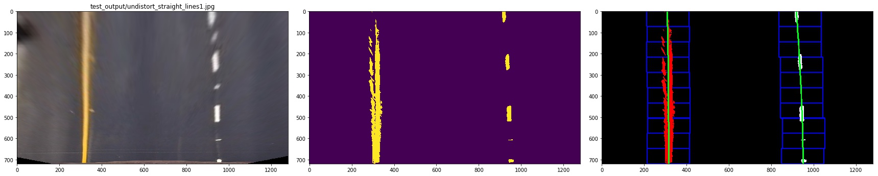
I plot the histogram of the bird-view image, then find the peek to decide the left base and right base of the lane lines

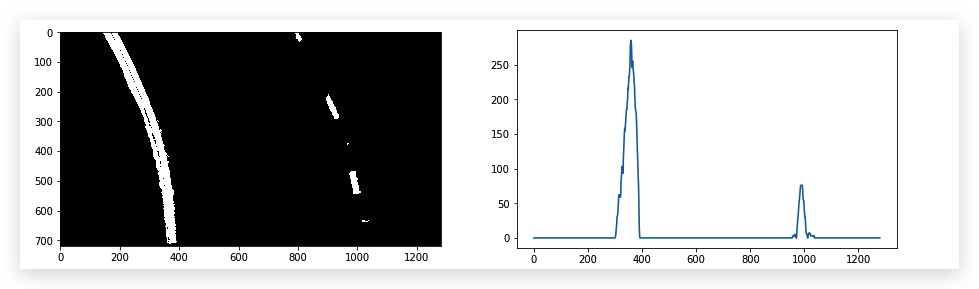
then we use slide window to find the lane pixels:

define 10 windows, the window's height is the height of image divide num of windows
loop through those windows
- Identify window boundaries in x and y (and right and left)
- Identify the nonzero pixels in the image and their index
- Identify the nonzero pixels in x and y within the window and append its index to each line
- If we found > minpix pixels, recenter next window, the new center is the mean of pixels' co
Extract left and right line pixel positions

find_lane_pixels

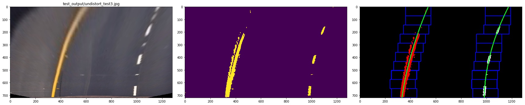
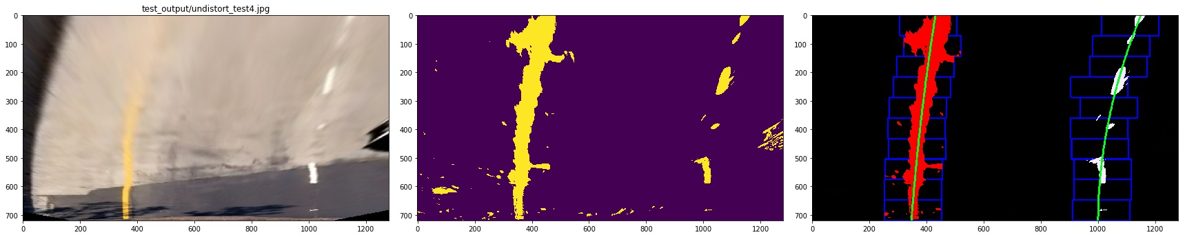
At last, we need to use polyfit function in numpy to find a line that is best fit the pixels of each line.

# Find our lane pixels first
leftx, lefty, rightx, righty, out_img = find_lane_pixels(binary_warped)
left_fit = np.polyfit(lefty, leftx, 2)
right_fit = np.polyfit(righty, rightx, 2)

we can use list comprehension to make (x,y)

pts_left=np.array([[x,y] for x,y in zip(left_fitx,ploty)],np.int32).reshape((-1,1,2))
pts_right=np.array([[x,y] for x,y in zip(right_fitx,ploty)],np.int32).reshape((-1,1,2))

but we can still use np.vstack to make (x,y)

left_line = np.array([np.transpose(np.vstack([left_fitx, ploty]))])

let me show you the result:

5. Describe how (and identify where in your code) you calculated the radius of curvature of the lane and the position of the vehicle with respect to the center.

First, we define the transformation rules to trans image pixels to real world length

ym_per_pix = 30/720 # meters per pixel in y dimension
xm_per_pix = 3.7/700 # 
lane_center_px_psp = 600

then we calculate the radius of curvature of the lane

left_curverad = ((1 + (2*left_fit_cr[0]*y_eval*ym_per_pix + left_fit_cr[1])**2)**1.5) / np.absolute(2*left_fit_cr[0])
right_curverad = ((1 + (2*right_fit_cr[0]*y_eval*ym_per_pix + right_fit_cr[1])**2)**1.5) / np.absolute(2*right_fit_cr[0])
center_offset = (((left_fit[0] * y_eval**2 + left_fit[1] * y_eval + left_fit[2]) + 
                   (right_fit[0] * y_eval**2 + right_fit[1] * y_eval + right_fit[2])) / 2) - lane_center_px_psp

center_offset = center_offset*xm_per_pix

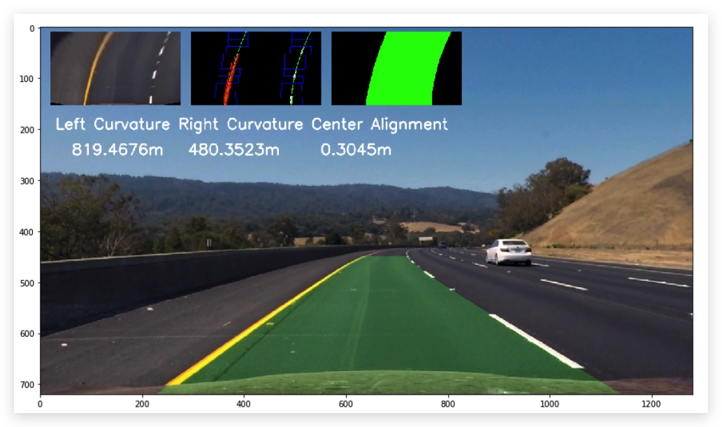
to see it clearly, I combined the image as below:

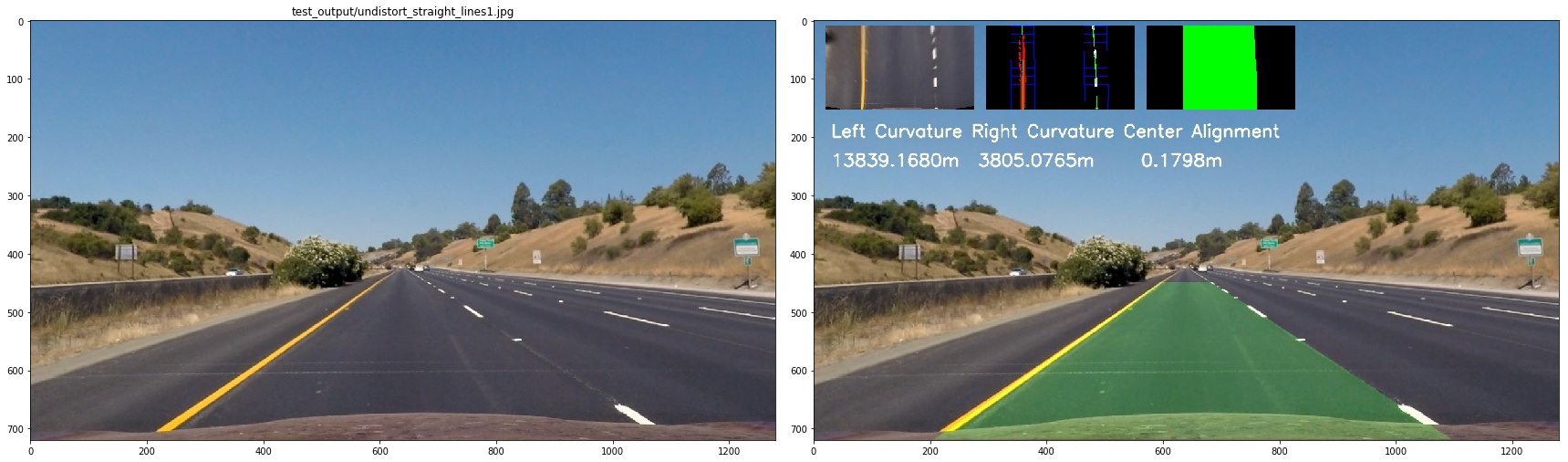
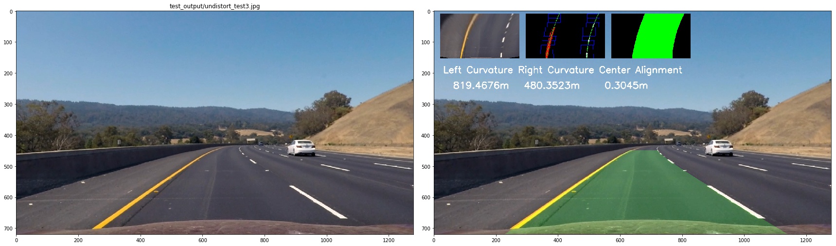
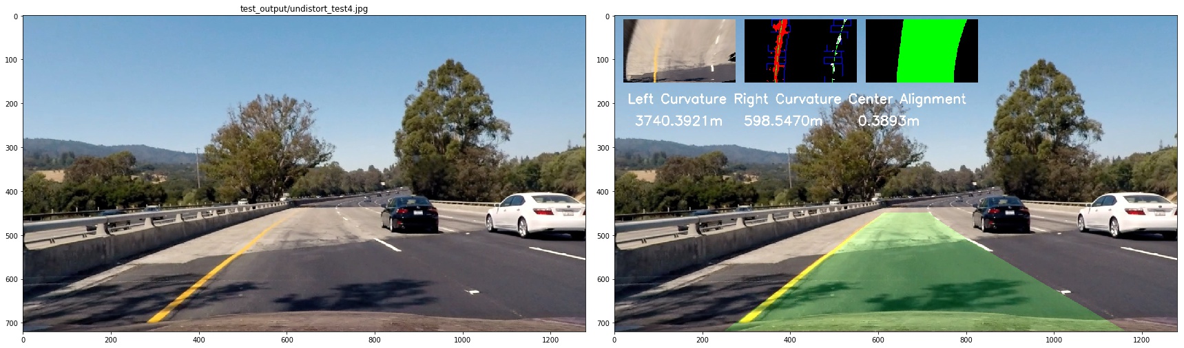
6. Provide an example image of your result plotted back down onto the road such that the lane area is identified clearly.

Pipeline (video)

1. Provide a link to your final video output. Your pipeline should perform reasonably well on the entire project video (wobbly lines are ok but no catastrophic failures that would cause the car to drive off the road!).

Here's a link to my video result

or this one

Discussion

1. Briefly discuss any problems/issues you faced in your implementation of this project. Where will your pipeline likely fail? What could you do to make it more robust?

Problems

it's hard to find the best threshold
the first time when I make perspectve transform , the order of src point and dest is not same, so the bird-view picture is actually up-side down but its hard to notice and it can infulence the result

What Could Be Improved

the algo that I used will failed on challenge_video.mp4,still have no idea how to fix it yet
I should explore more color space ,such as LAB
I think I should use prior infomation of the lane lines as I did in projet one

# Writeup

#Advanced Lane Finding Project

# Here I will consider the rubric points individually and describe how I addressed each point in my implementation.

# the implementation can be found here

# Camera Calibration

# 1. Briefly state how you computed the camera matrix and distortion coefficients. Provide an example of a distortion-corrected calibration image.

# 1. Prepared the object points and image points

# 2. Using those two points sets to calibrate camera:

# 3. Using the cv2.calibrateCamera return to undistort() the image

# 4. Then we apply the measurement to our test images

# Pipeline (single images)

# 1. Provide an example of a distortion-corrected image.

# 2. Describe how (and identify where in your code) you used color transforms, gradients or other methods to create a thresholded binary image. Provide an example of a binary image result.

# 1. We use sobel operator the take the gradient thresholds

# 2. Color Thresholding

# 3. Combine the gradient and color threshed

# 3. Describe how (and identify where in your code) you performed a perspective transform and provide an example of a transformed image.

# 4. Describe how (and identify where in your code) you identified lane-line pixels and fit their positions with a polynomial?

# 5. Describe how (and identify where in your code) you calculated the radius of curvature of the lane and the position of the vehicle with respect to the center.

# 6. Provide an example image of your result plotted back down onto the road such that the lane area is identified clearly.

# Pipeline (video)

# 1. Provide a link to your final video output. Your pipeline should perform reasonably well on the entire project video (wobbly lines are ok but no catastrophic failures that would cause the car to drive off the road!).

# Discussion

# 1. Briefly discuss any problems/issues you faced in your implementation of this project. Where will your pipeline likely fail? What could you do to make it more robust?

# Problems

# What Could Be Improved